Hide Data in Excel

Get FREE Advanced Excel Exercises with Solutions!

In this Excel tutorial, we will learn how to

– Hide the Entire row and column

– Hide data using different features from the toolbar

– Hide data using the Hide command and Format option.

– Apply conditional formatting to change the color and hide data

– Hide formulas and particular cell

Excel adds various features in different versions as a result all the features are not available in every version. However, all the methods used in this tutorial are available in Excel 2013, Excel 2016, Excel 2016, Excel 2019, Excel 2021, and Microsoft 365 versions.

Therefore, we will use hidden data in Excel for better visualization, a better way to analyze, and an easy way to protect confidential data.

Here is the overview image of this article, Follow more and go through the total article to know more about hiding data in Excel.

Table of Contents hide

What Are the Ways to Hide Data in Excel Using Keyboard Shortcut?

To hide data, here we will use the keyboard shortcut. But there are different shortcuts depending on rows or columns.

1. How to Hide Entire Row?

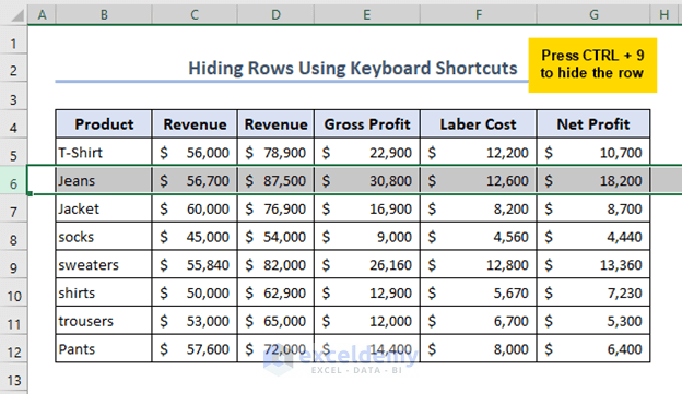
Therefore, in this method, we will hide the data of an entire row.

Initially, select the row by clicking on the row bar, then press CTRL + 9 to hide the data. Use 9 from the typing keys instead of the Neumeic keypad.

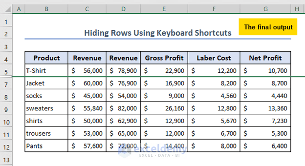
Finally, get the final output with a hidden row.

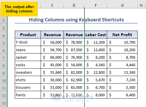
2. How to Hide the Entire Column?

Here, in this method, we will hide an entire column using the keyboard shortcut.

Select the column by clicking the column bar, and press CTRL + 0 to hide the data in the column. Therefore, select 0 from the typing keys instead of the numeric keypad.

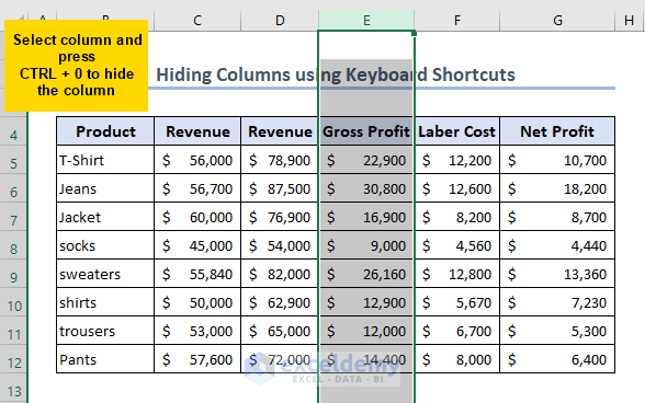
Once this process is complete, the final output will be similar to the one below.

What Are the Methods to Hide Data Using Toolbar in Excel?

To hide data in Excel using the Toolbar you can use four different methods. Now you can hide the data using any of these methods, as per your requirements.

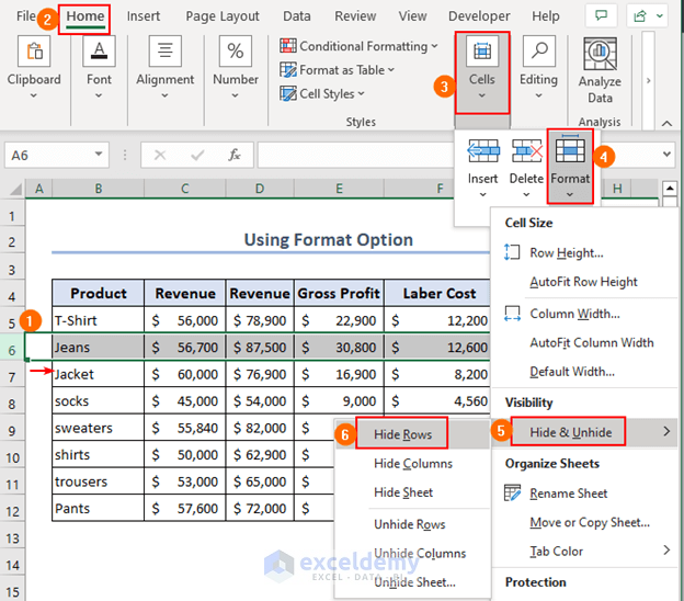
1. How to Use Format Group?

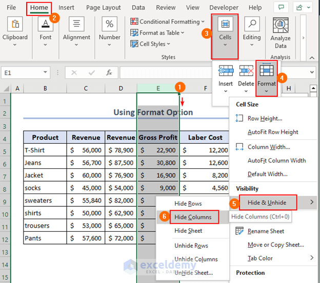
If you want to hide an entire column’s data then select the entire column and follow the below steps.

Initially, go to the Home tab >> Cells >> Format >> Hide & Unhide >> Hide Columns to hide the entire column.

To hide the entire row’s data, follow the steps already shown here, but instead of selecting Hide Columns from the Format dropdown, select Hide Rows to hide the entire row.

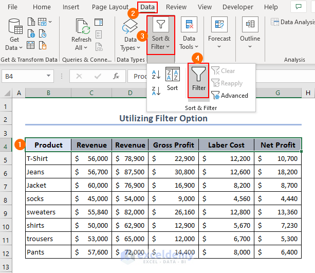
2. How to Apply Filter Command?

There is an option in Excel called “Filter” and you can filter any sort of data using this option.

Select the heading cells from the dataset and click the Data tab >> Sort & Filter >> Filter as below.

Open the filter option from Gross Profit and select the data that will be visible.

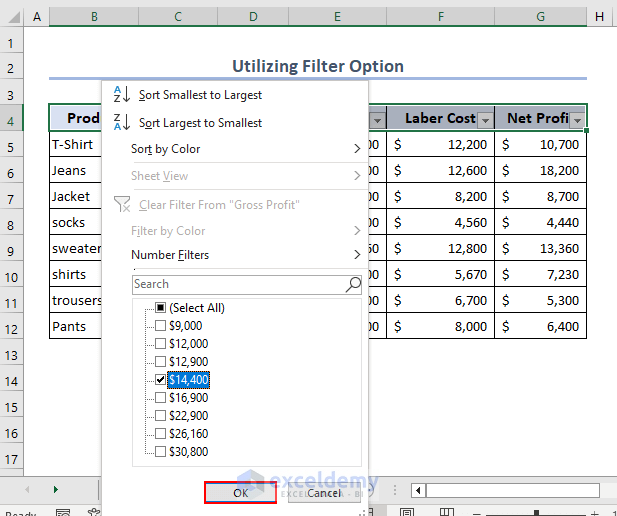
Finally, click OK to complete the process. Once the process is complete the data will be hidden but the hidden data will be still in the dataset.

3. How to Apply the Advanced Filter Option?

There is another option, which is the Advanced Filter. With this option, the data can be filtered according to criteria. Suppose you need to hide all the data where the net profit is less than $10,000.

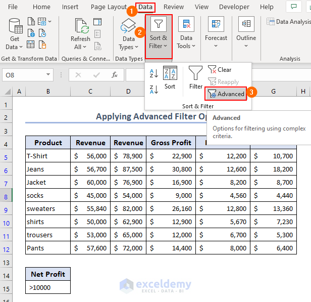
Now click on the Data tab >> Sort & Filter >> Advanced Filter.

The Advanced Filter dialog box will open. Select list range B4:G12 and Criteria range B14:15.

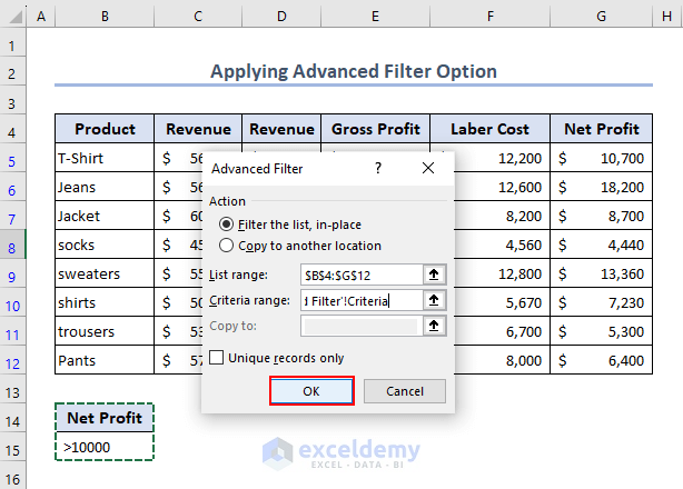
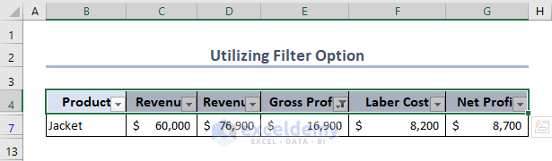
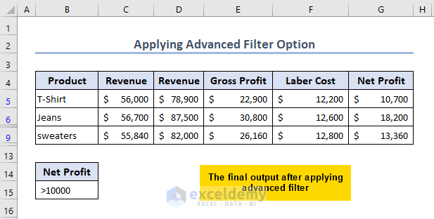
Finally, click OK to complete the process, and the final output will show only the data with more than $10,000 in net profit.

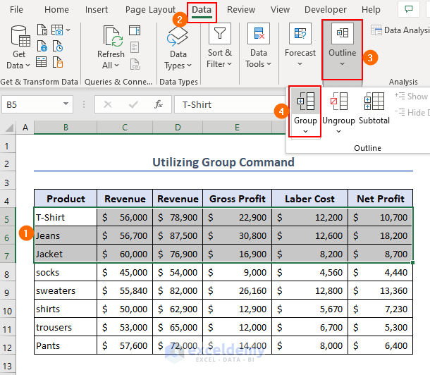
4. How to Use Group Command?

Here, In this method, we will create a group and hide the data in Excel.

To create a group, select the cells and go to the Data tab >> Outline >> Group as below.

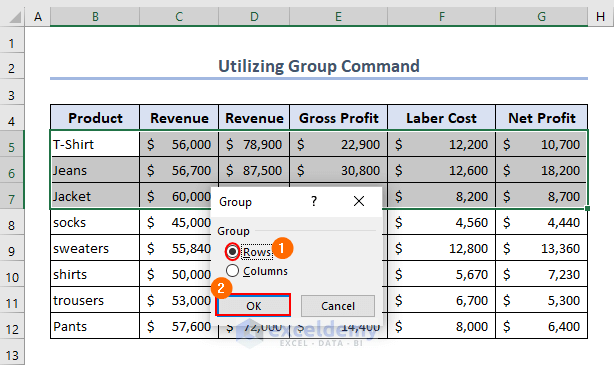
The Group dialog box will open up and allow you to select rows if the group is row-wise or columns if the group is column-wise.

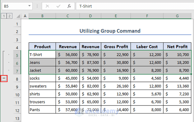
Now, to hide the entire group, click on the (-).

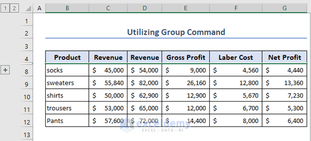
Once the full process is done, the final output with the hidden data will be below.

Read More: How to Hide Part of Text in Excel Cells

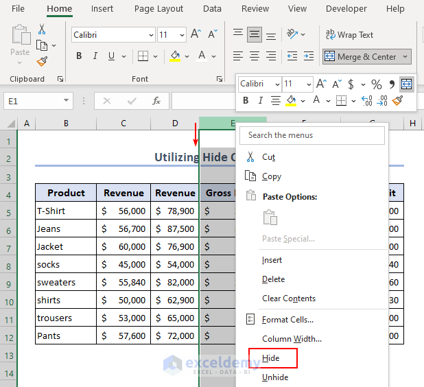
How to Hide Data Using Hide Command in Excel?

You can hide the required data using the options bar as well. There are different methods for executing the processes. To hide data, use the Hide command in Excel as below.

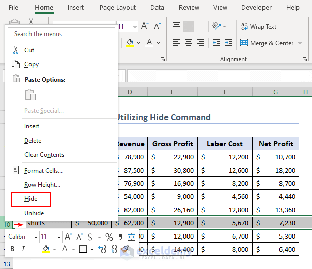
Select the column and right-click the mouse to open the options bar. Select the Hide option to hide the data.

Note: You can hide an entire row using the same process.

What Are the Methods to Hide Confidential Data in Excel?

To hide the confidential data in Excel you can use 5 methods. Once you protect the sheet, it is unchangeable. So, these processes are safer and more accurate.

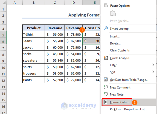
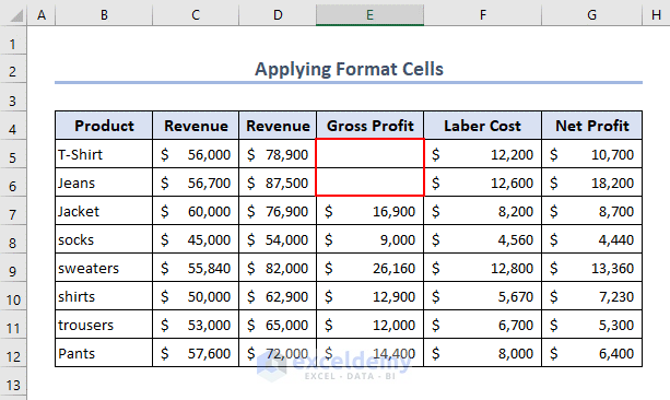
1. How to Apply Format Cells?

Therefore, we will learn how to apply format cells in Excel to hide data.

Initially, select the cell and right-click on the mouse. Then the options bar will open, and select Format cells as below.

Now, write down (;;;) in the type option and click on OK.

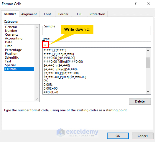
After completing the process, the cells will be hidden as below.

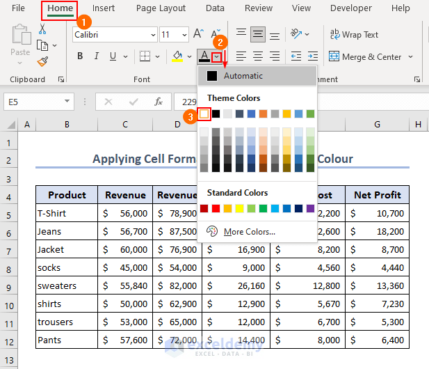
2. How to Apply Cell Formatting to Change Font Color?

Here, in this method, we will learn how to hide data by applying cell formatting to change color.

To change the Text font color to hide the data in a particular cell, go to the Home tab and click on the drop-down menu in the font section.
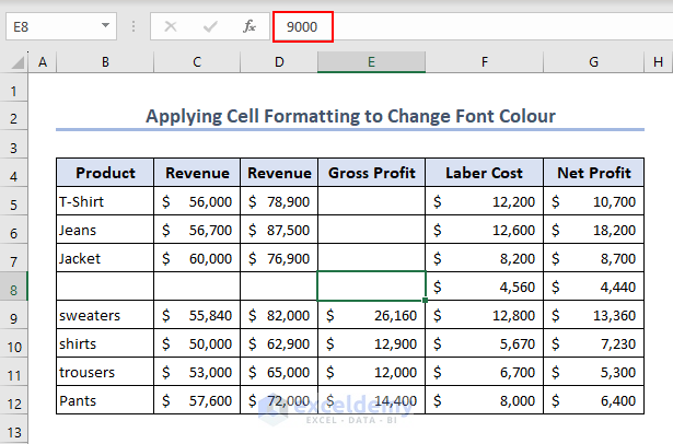
Select White so that the text color matches the background and no data is visible.

However, after selecting the cell, the hidden data will be visible in the formula bar as below.

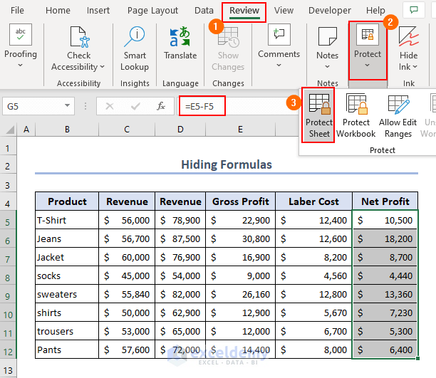
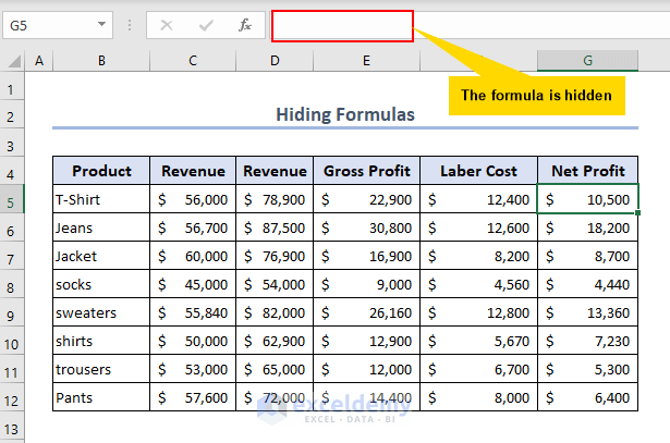
3. How to Hide Formulas?

Therefore, we will hide formulas in this method.

Initially select the cell and open the Format cell.
Then go to Protection >> Locked and Hidden >> OK to lock and hide the cells. But this option will not activate unless the sheet is protected.

Now, protect the sheet by clicking Review >> Protect >> Protect Sheet.

After that, select a password and click OK.
Lastly, confirm the password and that the sheet is protected.

Finally, the sheet is protected, and the formula is hidden in the formula bar.

4. How to Hide Particular Cells?

Sometimes we need to hide particular cells in Excel, and this process is the most critical to execute. Now, follow the steps below to hide particular cells in Excel in an easy way.

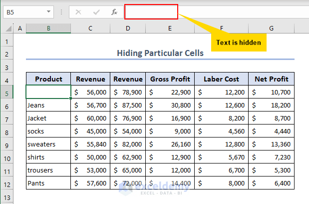
Select the cell and change the font color to white to hide.

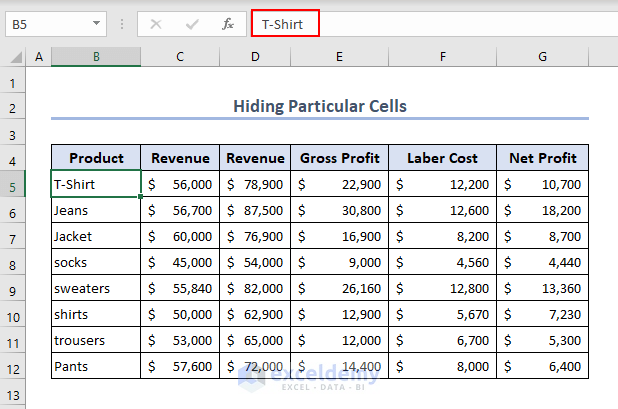
Open the format cell option lock and hide the cell to hide the text from the formula bar as well.

Similar Readings

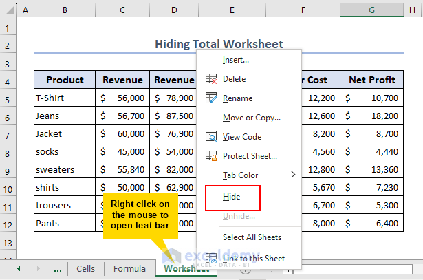
5. How to Hide Total Worksheet?

Now, we will hide the total worksheet in Excel using the below process.

Initially, lock the entire sheet using the process already shown before.
Then, right-click on the leaf bar and select Hide from the bar to hide the entire sheet.

Things to Remember

Protect the sheet after you hide any data so that the data remains unchanged.
Always keep a backup of the original data, just to be safe.
If you use Excel simple or direct option then you can not hide selected data in Excel. In that case, you need to hide or unhide an entire row or column.
You get better visualization after hiding data from the dataset. however you print the dataset you will get to see the hidden data on the printed copy.

Frequently Asked Questions

Q1: Will hidden data permanently be removed in Excel?

Ans: No, hidden data is not removed from Excel. You can easily unhide the data and continue.

Q2: How to unhide cells in Excel?

Ans: Once you hide the cells, you need to unhide them. Select CTRL + SHIFT + 9 to unhide cells row-wise and press CTRL + SHIFT + 0 to unhide cells column-wise.

Q3: How do I print with hidden data?

Ans: If you print with hidden data, then the data will be shown in the printed sheet. So, print in the normal procedure to get the hidden data.

Download Practice Workbook

Hide Data.xlsx

Conclusion

From this article, we have learned how to hide data in Excel in different ways, such as applying keyboard shortcuts, the toolbar, the Filter option, the Advanced Filter option, the Hide command, and the options bar. Here, we covered every possible way to hide data, especially if the data is confidential. These methods are very helpful. Hopefully, you can solve the problem shown in this article. Please let us know in the comment section if there are any queries or suggestions.