Microsoft Excel is a powerful software. We can perform numerous tasks on datasets using Excel tools and features. There are many default Excel functions that we can use to create formulas. Many educational institutions and business companies use excel files to store valuable data. Often, we have to estimate a quantity for producing a product. We estimate such figures based on market demands. However, the demands don’t stay consistent. Thus, we take the probability into account for each quantity. We can simulate the probability easily in excel. This article will show you step-by-step procedures to get Simulation Probability in Excel.
How to Get Simulation Probability in Excel: Step-by-Step Procedures
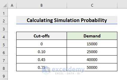
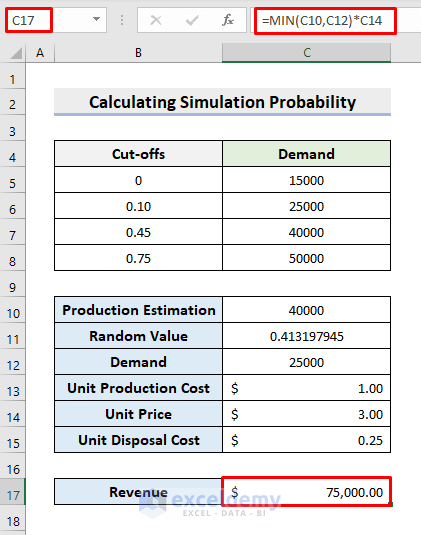
We’ll consider a case in this example. Suppose we have to estimate a quantity to manufacture a product. In this regard, we set up the Demand and Cut-offs values. To illustrate, we’ll use the following dataset. For instance, the dataset considers random values from 0 to less than .10 to fall under the demand of 15000, from .10 to less than .45 to fall under 25000, from .45 to less than .75 to fall under 40000, and random values equal to .75 and above fall under 50000. Now, we’ll perform a simulation probability for picking a quantity to produce so that we earn maximum profit and have the minimum amount of unsold products simultaneously.
STEP 1: Input Estimation
- First, we’ll estimate a quantity for production.
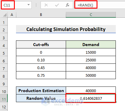
- Type the quantity in cell C10.

STEP 2: Generate Random Value
- Then, select cell C11.
- Here, input the formula:
=RAND()- Subsequently, press Enter.
- The RAND function generates random values.
STEP 3: Simulate Demand
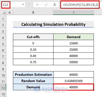
- Now, we’ll extract the demand against the random number in cell C11.
- For this purpose, choose cell C12.
- Insert the formula:
=VLOOKUP(C11,B5:C8,2)- Hit Enter.
- The VLOOKUP function searches for the C11 cell value in the range B5:C8 and returns the value from the 2nd column i.e. Demand.
Read More: How to Calculate Empirical Probability with Excel Formula
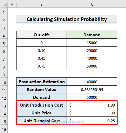
STEP 4: Insert Necessary Info
- Afterward, we’ll input necessary info like Unit Production Cost, Price, and Disposal Cost in the range C13:C15.
STEP 5: Create Required Formulas
- Firstly, we’ll determine the Revenue.
- So, click cell C17.
- Next, type the formula:
=MIN(C10,C12)*C14- Press Enter.
- The MIN function gives out the minimum quantity between cells C10 and C12.
- Now, to get the total production cost, select cell C18.
- Insert the formula:
=C10*C13- Click Enter.

- For calculating the total disposal cost, choose cell C19.
- Input the formula:
=C15*IF(C10>C12,C10-C12,0)- After that, press Enter.
- The IF function tests whether the estimated quantity is greater than the demand.
- Only then, there will be a disposal cost.
- Otherwise, the disposal cost will be 0.

- Finally, to get profit, click cell C20.
- Type the formula:
=C17-C18-C19- Subsequently, press Enter.

Read More: Probability Formula for Lottery in Excel
STEP 6: Set up Dataset
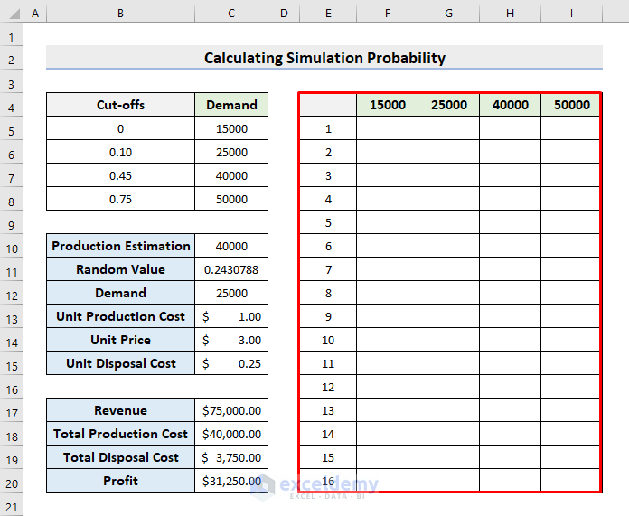
In this step, we will set up the worksheet for performing the simulation.
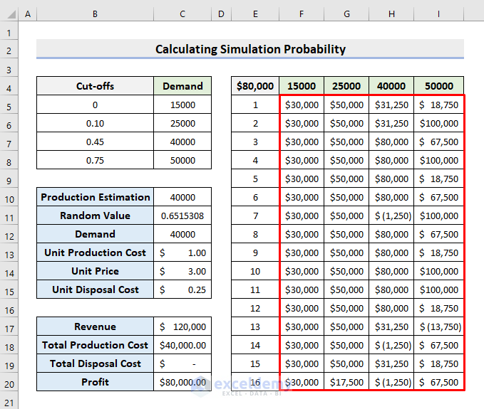
- First of all, set up the dataset in the range E4:I20.
- Input each of the quantities in the range F4:I4.
- Look at the picture below for a better understanding.
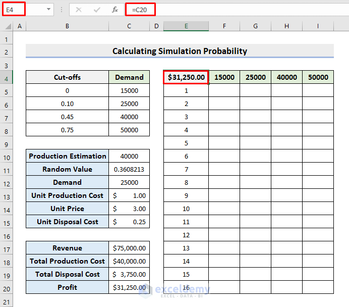
- Then, select cell E4.
- Here, we’ll input the profit amount.
- Hence, type the formula:
=C20- Press Enter.
STEP 7: Perform Probability Simulation
In this step, we’ll perform the iteration. For any kind of simulation probability, a larger number of iterations are always recommended. However, in this example, we will conduct 16 iterations for demonstration convenience. Therefore, follow the process.
- After that, select the range E4:I20.
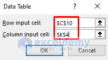
- Next, go to Data > Forecast > What-If Analysis > Data Table.
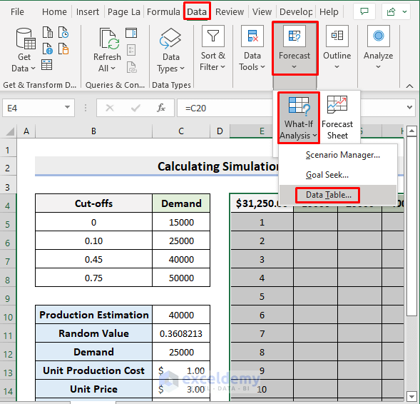
- As a result, the Data Table dialog box will pop out.
- Select cell C10 as the Row input cell and any blank cell, for example, K4 as the Column input cell.
- Afterward, press OK.
- Accordingly, it’ll return the calculated profit amounts for each of the product quantities.
- See the following figure to clearly understand.
Read More: How to Apply Weighted Probability in Excel
STEP 8: Simulate Best Probable Result
Now, we have to pick the best probable quantity to produce, considering the profits and disposal costs too. So, learn the process.
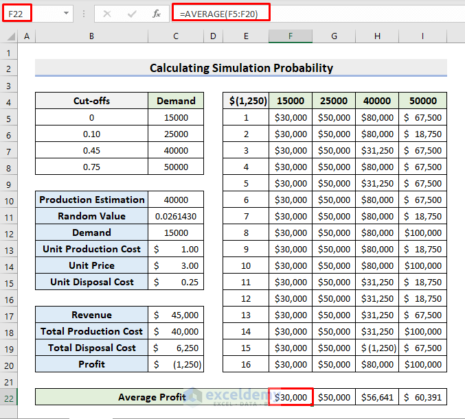
- In the beginning, select cell F22.
- Type the formula:
=AVERAGE(F5:F20)- Press Enter.
- Subsequently, use AutoFill to the right.
- The AVERAGE function computes the average of the profits for each quantity.
- Moreover, to get the Standard Deviation, click cell F23.
- Insert the formula:
=STDEV(F5:F20)- Hit Enter and apply AutoFill.
- The STDEV function computes the standard deviation.
- In this way, we’ll get the deviation.
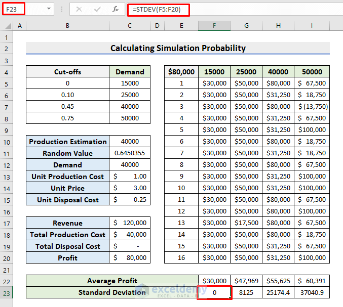
- Notice, there is no standard deviation for 15000. That means, there will be no leftovers.
- Consequently, if you do a higher number of iterations, you’ll get one quantity which will always yield the maximum profit.
- Again, to avoid any risks, consider picking the amounts which have lower risks.
- In such a process, you can calculate the simulation probability.
Download Practice Workbook
Download the following workbook to practice by yourself.
Conclusion
Henceforth, you will be able to get simulation probability in Excel by following the above-described steps. Keep using them and let us know if you have more ways to do the task. Don’t forget to drop comments, suggestions, or queries if you have any in the comment section below.
Related Articles
- How to Calculate Probability Density Function in Excel
- How to Create Option Probability Calculator in Excel
- How to Make a Probability Tree Diagram in Excel
<< Go Back to Excel Probability | Excel for Statistics | Learn Excel
Get FREE Advanced Excel Exercises with Solutions!
