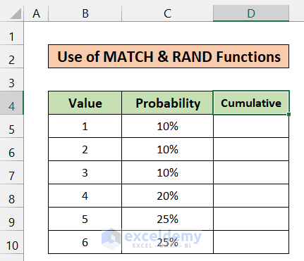
Method 1 – Combining MATCH and RAND Functions to Apply Weighted Probability in Excel
Steps:
- Create a new Cumulative column.
- On cell D5, the cumulative will be 0. But on cell D6, it will be the sum of C5. Put the following formula in cell D6.
=SUM(C5,D5)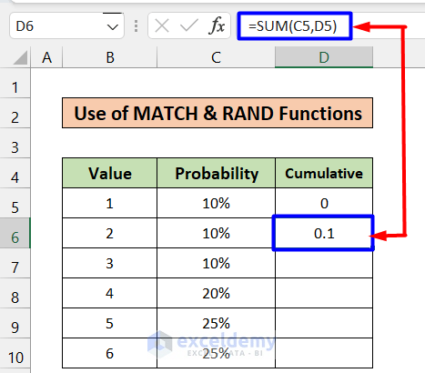
- Use the Fill Handle to copy the formula into the rest of the cells on the cumulative column.
- To generate a random number, take another column and name it Results.
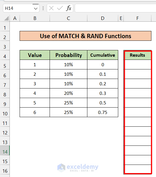
- In cell F5, use the following formula and press Enter. You should get a number between 1 to 6.
=MATCH(RAND(),$D$5:$D$10)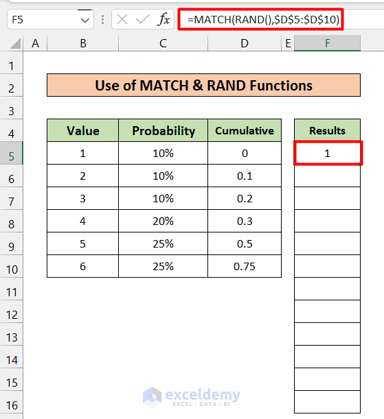
- We will again use Fill Handle to copy the formula into the other cells below.
- Since we have used the RAND function, the values obtained now will be changed if any further operation is performed. To prevent changing values, we can copy and paste the values. We will lose the formula on the cells, but they will not get changed in the future.
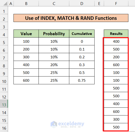
- The final result should be like this.
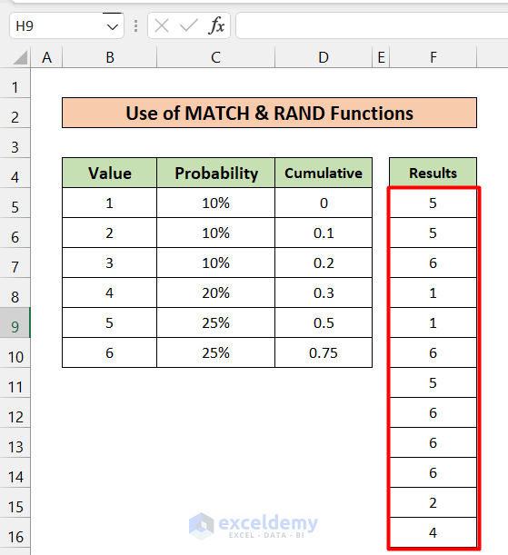
- As we have taken only a small number of cells, the frequency of getting a number does not entirely obey the assigned probability. If we generate a large set of numbers, the frequency will be very close to the assigned probability.
How Does the Formula Work?
- RAND()
The RAND function generates a random number between 0 and 1.
- MATCH(RAND(),$D$5:$D$10)
The MATCH function takes the first argument from the RAND function and searches the value in the range of D5:D10(Cumulative column). It returns the largest row number where the value on the Cumulative column<=searched value.
Note:
- The numbers must be arranged in ascending order in the Value
- The return value of the MATCH function is the same as the numbers to be randomly generated. If this is not the case, we can not use this method. As a result, we have to use the 2nd method.
Method 2 – Apply Weighted Probability in Excel Utilizing INDEX, MATCH & RAND Functions
Steps:
- In cell F5, use the following formula and click the Enter key.
=INDEX($B$5:$B$10,MATCH(RAND(),$D$5:$D$10))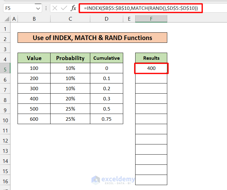
- Autofill the rest of the cells.
How Does the Formula Work?
- MATCH(RAND(),$D$5:$D$10))
Like the 1st method, MATCH(RAND(),$D$5:$D$10)) will yield integer values ranging from 1 to 6. This value will be passed as 2nd argument of the INDEX function.
- INDEX($B$5:$B$10,MATCH(RAND(),$D$5:$D$10))
The formula as a whole will return the cell value from the Value column(B5:B10) corresponding to the row number passed by the MATCH function.
Note:
- The values we want to generate randomly are not mandatory to be numerical only. They can be text as well.
Method 3 – Using INDEX, COUNTIF, and RAND Functions
Steps:
- In cell F5, use the following formula
=INDEX($B$5:$B$10,COUNTIF($D$5:$D$10,"<="&RAND())+1)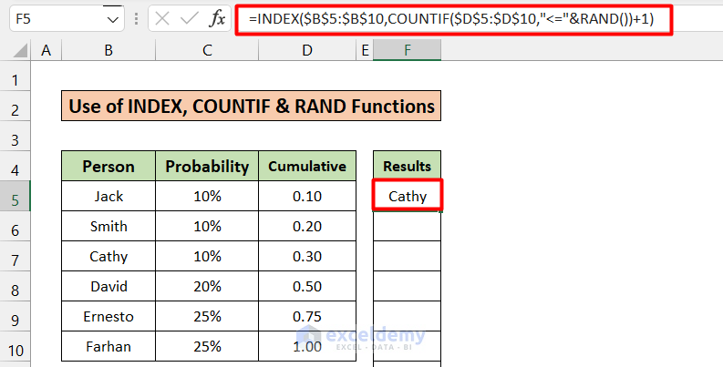
- If we autofill the formula for the rest of the cells, we will get the following results.
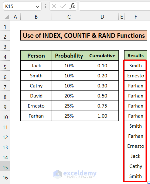
- From the above figure, it is evident that the person with a larger probability weightage has appeared more often than the lesser ones.
How Does the Formula Work?
- RAND()
This function generates a random number between 0 and 1
- RAND())+1
This adds 1 with the randomly generated value.
- COUNTIF($D$5:$D$10,”<=”&RAND())+1)
It counts the number of cells in the Cumulative column(D5:D10) that are less than RAND())+1
- INDEX($B$5:$B$10,COUNTIF($D$5:$D$10,”<=”&RAND())+1)
It returns the cell value of column Person(B5:B10) corresponding to the row number taken as the 2nd argument of the INDEX function.
Things to Remember
- The 1st method is only applicable if the row numbers and the set of generated numbers are the same.
- 2nd and 3rd are applicable for both generating numerical and numerical values.
- The 3rd method has a different way of calculating the Cumulative column.
Download the Practice Workbook
Related Articles
<< Go Back to Excel Probability | Excel for Statistics | Learn Excel
Get FREE Advanced Excel Exercises with Solutions!
