A diagram that is used to provide a visual depiction of the possibilities and outcomes of an event is called a probability tree diagram. Using Microsoft Excel, we can easily do such work. In this article, we are going to demonstrate 3 handy ways to make a probability tree diagram in Excel. If you are also curious about it, download our practice workbook and follow us.
Overview of Probability Tree
A diagram that is used to provide a visual depiction of the possibilities and outcomes of an event is called a probability tree diagram. The nodes and branches make up the two components of the tree diagram. An event is represented by a node. A branch is a visual representation of the relationship between an event and its result.
For example, we can consider a coin that has two sides: a head and a tail. If we toss the coin, it can either come head or tail. The calculated probability of getting anyone will be 0.5 or 50%. Now, if we show this scenario in the probability diagram tree, that will be like the image shown below:

How to Make a Probability Tree Diagram in Excel: 3 Easy Ways
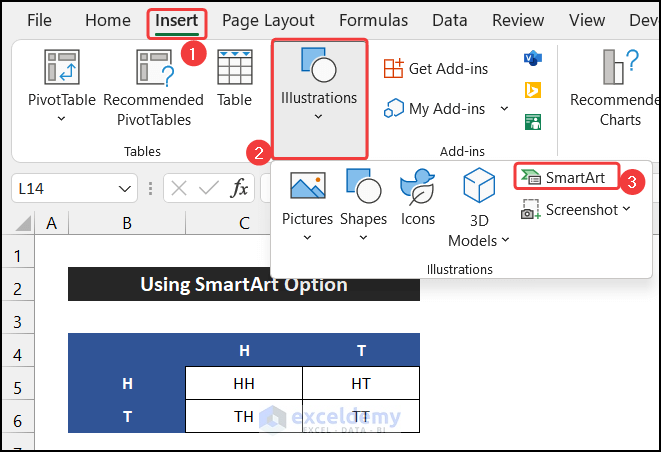
To demonstrate the approaches, we take a coin and toss it twice. As a result, we get the four combinations of the events that can occur during the toss. We show the possible events in the range of cells C5:D6.

📚 Note:
All the operations of this article are accomplished by using Microsoft Office 365 application.
1. Using SmartArt Option to Create a Probability Tree Diagram
In this method, we are going to use the SmartArt option to make a probability tree diagram in Excel. The steps of this process are given below:
📌 Steps:
- First of all, go to the Insert tab.
- Now, click on the drop-down arrow of the Illustration and choose the SmartArt option.
- As a result, a small dialog box called Choose a SmartArt Graphic will appear.
- Then, from the Hierarchy tab, choose a chat according to your desire. We chose the Horizontal Organization Chart.
- Finally, click OK.

- The chart will appear on the spreadsheet.

- Here, when we toss the coin first time, we will get either head or tail. So, format the chart as two possible events that can come from an event.

- After that, from each event, we will get two more events.
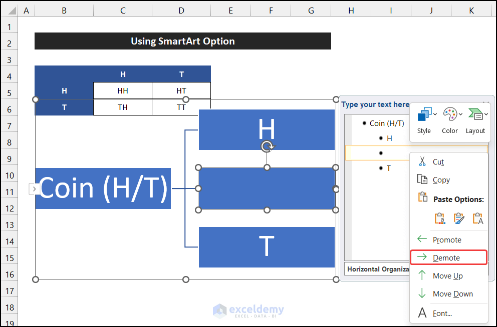
- To insert them, click on the right arrow on the right side of the chart.
- As a result, a small side window will appear.

- Now, press Enter to add another point after H or head.
- Then, right-click on the point and select the Demote option to create the section from the second toss.
- Afterward, write down the possible events in those boxes.

- Similarly, create another secondary section for the T or tail.

- At last, format the diagram according to your desire.
- Our probability tree is ready.

Thus, we can say that our procedure works perfectly, and we are able to make a probability tree diagram in Excel.
Read More: Probability Formula for Lottery in Excel
2. Make a Probability Tree Diagram Utilizing the Shapes Option from Insert Tab
In this process, we will use the Shapes to make a probability tree diagram in Excel. The procedure of this process is described below step-by-step:
📌 Steps:
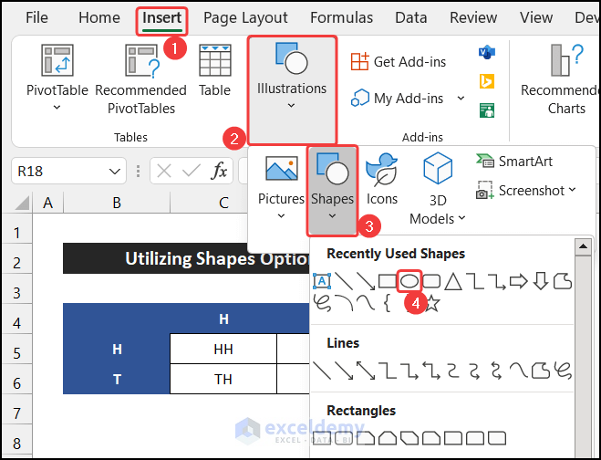
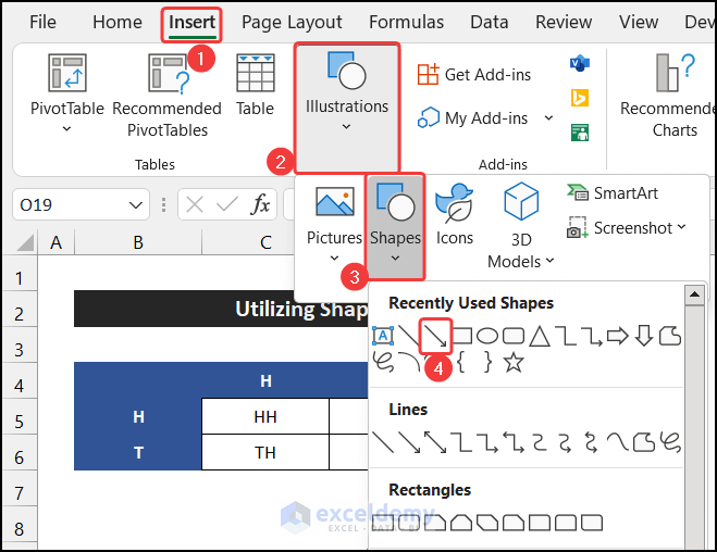
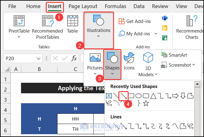
- First, in the Insert tab, click on the drop-down arrow of the Illustration > Shapes option.
- Then, click on a shape according to your desire. Here, we choose the Oval shape.
- You will notice that your mouse cursor look will change.
- Now, click on the empty place and drag the mouse to get the shape.
- Then, resize the shape according to your need.

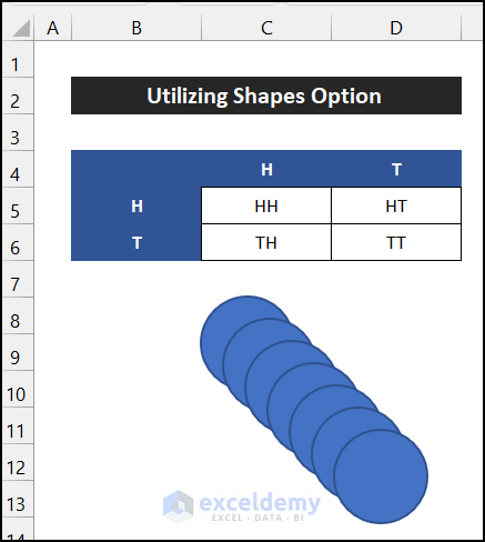
- We know that in the first toss, we can get two identical events, and after the second toss, the number of events will go to four.
- So, press ‘Ctrl+D’ six times to create a similar type of oval 6 times. These ovals are the nodes of the probability tree diagram.
- After that, rearrange them into 1, 2, and 4 in order and write down the following events.

- Now, we have to insert the branch. For that, again, go to the Insert tab.
- Then, click on the drop-down arrow of the Illustration > Shapes option and choose the Line Arrow shape.
- Insert the Line Arrow shape as we insert the Oval shape.

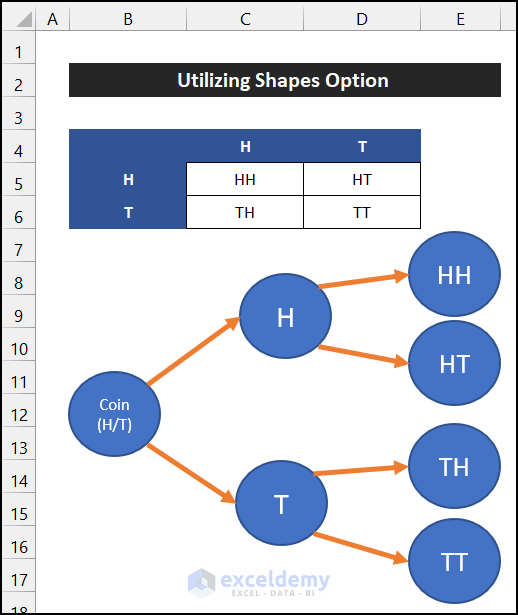
- At last, place the arrow to make a relation among the nodes like in the image shown below.

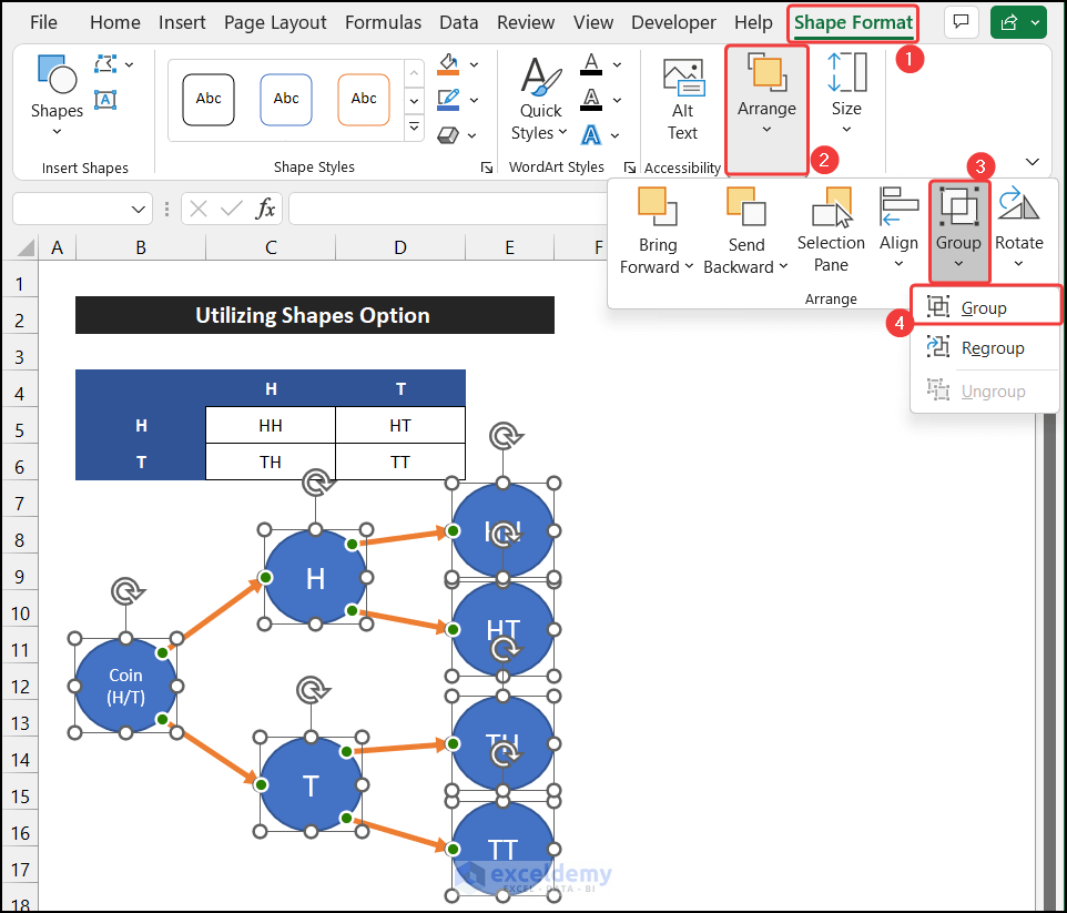
- Finally, format them according to your desire. Moreover, select all the shapes and click on the drop-down arrow of the Group > Group option from the Arrange group, located in the Shape Format tab, to stop their accidental movement.
- Our probability tree diagram is ready.
Hence, we can say that our approach works effectively, and we are able to make a probability tree diagram in Excel.
3. Applying the Text Box Feature to Make a Probability Tree Diagram
In the last approach, we are going to use the Text Box of Excel to make a probability tree diagram in Excel. The steps of this procedure are given as follows:
📌 Steps:
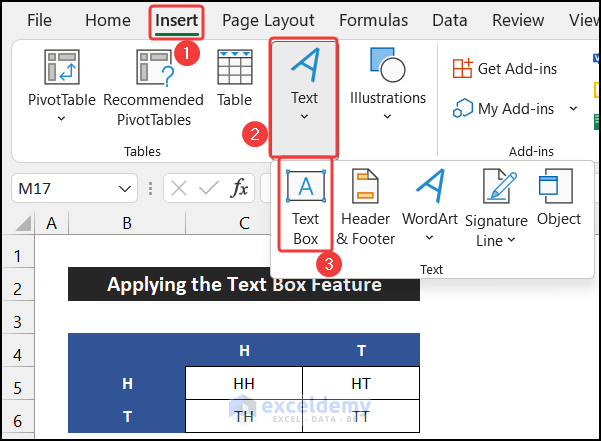
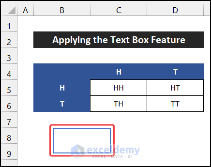
- At first, in the Insert tab, click on the drop-down arrow of the Text command and choose the Text Box option.
- You will see that your mouse cursor look will change.
- After that, click on the empty place and drag the mouse to get the text box.
- The box will appear on the sheet.
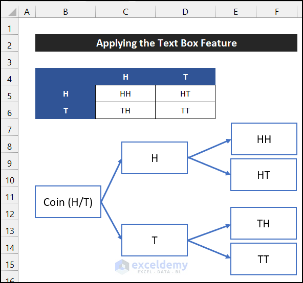
- We know that after the first toss, we will get two identical events, and after the second toss, the number of events will go to four.
- Thus, press ‘Ctrl+D’ six times to make a similar type of text box 6 times. Here, these text boxes are the nodes of the probability tree diagram.
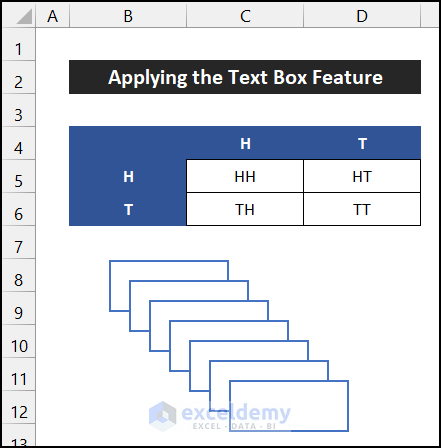
- Now, rearrange them into 1, 2, and 4 in order and write down the following events.
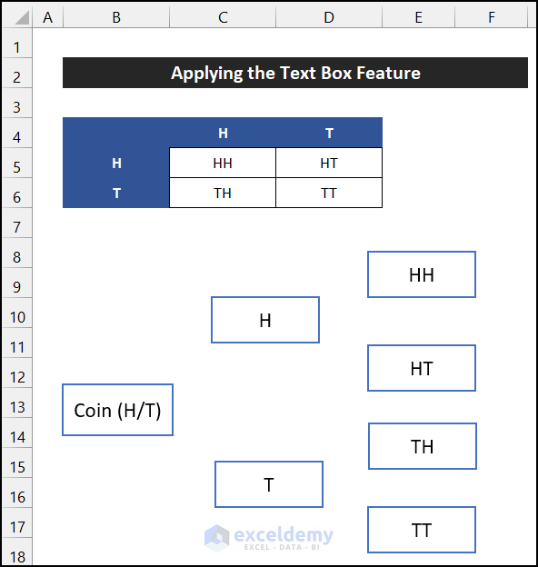
- Next, we have to insert the branch. To insert them, again, go to the Insert tab.
- Then, click on the drop-down arrow of the Illustration > Shapes option and choose the Line Arrow shape.
- Insert the Line Arrow shape as we insert the Text Box.

- In the end, place the arrow to make a relation among the nodes like in the image shown below.
- Afterward, format them according to your desire.
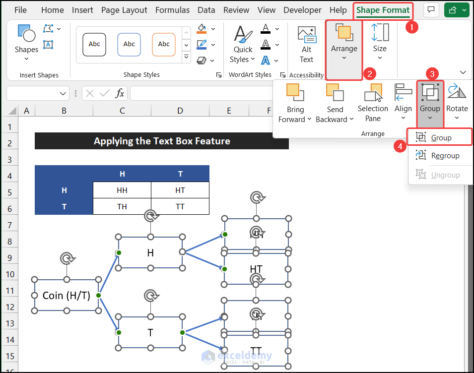
- In addition, select all the shapes and click on the drop-down arrow of the Group > Group option from the Arrange group, located in the Shape Format tab, to stop their accidental movement.
- Our probability tree diagram is ready.
Finally, we can say that our method works successfully, and we are able to make a probability tree diagram in Excel.
Download Practice Workbook
Download this practice workbook for practice while you are reading this article.
Conclusion
That’s the end of this article. I hope that this article will be helpful for you and you will be able to make a probability tree diagram in Excel. Please share any further queries or recommendations with us in the comments section below if you have any further questions or recommendations.
Related Articles
- How to Apply Weighted Probability in Excel
- How to Create Option Probability Calculator in Excel
- How to Get Simulation Probability in Excel
- How to Calculate Probability Density Function in Excel
- How to Calculate Empirical Probability with Excel Formula
<< Go Back to Excel Probability | Excel for Statistics | Learn Excel
Get FREE Advanced Excel Exercises with Solutions!
