While applying the Excel formula, we frequently use the cell address or cell reference to return a cell value. But if you work on an Excel sheet of a large amount of data and looking for a cell with specific text in it, you need to go through a large amount of data. But that’s not a smart approach and at the same time, it is very time-consuming. But don’t worry at all. In this article, I will show you how to return the cell address instead of the value in Excel.
How to Return Cell Address Instead of Value in Excel: 5 Ways
Let’s say we have a dataset of some information about some employees of different companies such as their names, email, IP address, etc.
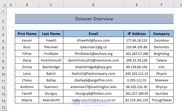
From this dataset, we want to return the cell address from a specific cell value.
In this section, you will find 5 common ways to return the cell address instead of value in Excel. I will demonstrate them one by one here. Let’s check them now!
1. Using ADDRESS and Match Functions
Let’s say, we have randomly chosen a cell value “Ambrosi”. The concerning dataset got the email addresses of the persons. We want to know the email address of “Ambrosi” and for this, we need to know the cell address in which the corresponding email id is located.
In order to find out the cell address, we will create a formula by using the ADDRESS and MATCH functions.
The MATCH function looks for a value in a defined lookup array for either an exact match or greater/less than the lookup value. The ADDRESS function gives the row and column number.
Proceed with the following steps to figure it out.
📌 Steps:
- First of all, select a cell to find out the cell address and type the following formula into the cell.
=ADDRESS(MATCH("Ambrosi",B5:B14,0),4)
Here,
- Ambrosi = lookup value
- B5:B14 = lookup array
- 0 = for the exact match
- 4 = column number (email address)
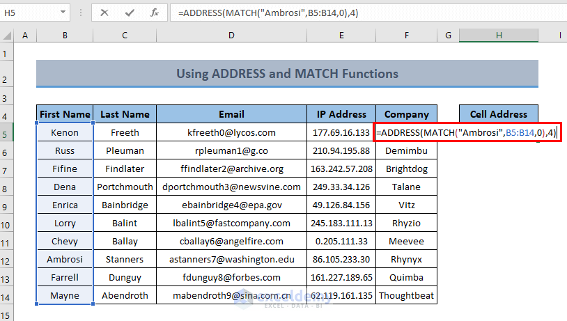
- Then, hit ENTER and you will get the cell address of the referenced cell value.

💡 Formula Breakdown
MATCH(“Ambrosi”,B5:B14,0) looks for an exact match of the value “Ambrosi” in the lookup array B5:B14 and finds the value in row number 8.
Output=> 8
ADDRESS(MATCH(“Ambrosi”,B5:B14,0),4) = ADDRESS(8,4)
We want to get the email address of Ambrosi and the email address is in column 4. And the MATCH function returns row number: 8
So, final Output=> $D$8

Read More: Excel VBA to Find Cell Address Based on Value
2. Combining CELL, INDEX and MATCH Functions
For the same set of data and the same lookup value (Ambrosi), we now create a formula by combining CELL, INDEX, and MATCH functions.
The INDEX function returns the cell reference at the intersection of a specific row and a column, The CELL function gives specific information (address, color, content, filename, format, etc.) about a referred cell.
In order to demonstrate this formula, just follow the steps below.
📌 Steps:
- Firstly, type the following formula in a selected cell to get the address.
=CELL("address",INDEX($B$5:$F$14,MATCH("Ambrosi",$B$5:$B$14,0),4))
Here,
- Ambrosi = lookup value
- B5:B14 = lookup array
- 0 = for the exact match
- 4 = column number (email address)
- address = info_type (the characteristic of the CELL function to return)
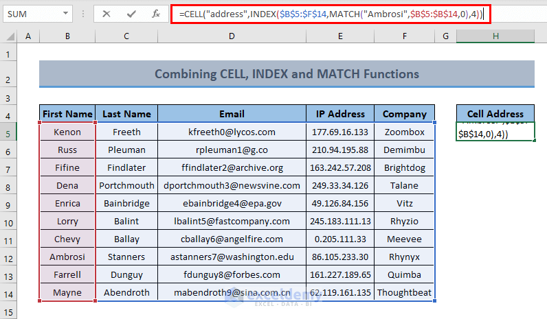
- Then, press ENTER to let the cell show the cell address instead of the cell value for the corresponding referred value.

💡 Formula Breakdown
MATCH(“Ambrosi”,B5:B14,0) looks for an exact match of the value “Ambrosi” in the lookup array B5:B14 and finds the value in row number 8.
Output=> 8
INDEX($B$5:$F$14,MATCH(“Ambrosi”,$B$5:$B$14,0),4) = INDEX($B$5:$F$14,8,4) returns the cell value at the intersection row 8 and column 4. These numbers are rows and columns of the corresponding dataset, not the Excel built-in dataset.
Output=>86.105.233.30
Finally, CELL(“address”,INDEX($B$5:$F$14,MATCH(“Ambrosi”,$B$5:$B$14,0),4)) = CELL(“address”,INDEX($B$5:$F$14,8,4)) = CELL(“address”,86.105.233.30) returns the address of 86.105.233.30.
So, final Output=> $E$12
Read More: Example of Cell Address in Excel
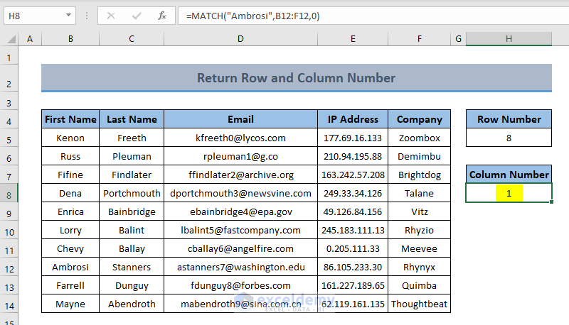
3. Return Row and Column Number Instead of Value
If you want to find out the row and the column number of the concerned dataset but not the Excel built-in row and column, then you can follow this procedure. For this, just proceed with the steps below.
📌 Steps:
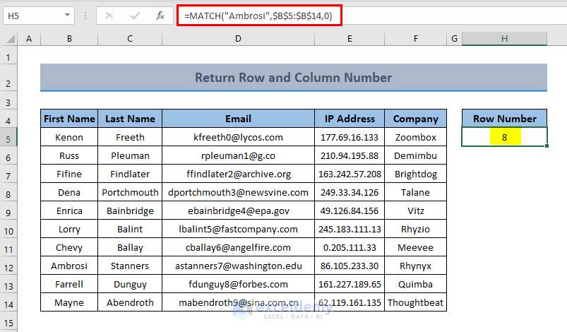
- First of all, apply the following formula to get the row number.
=MATCH("Ambrosi",$B$5:$B$14,0)
Here,
- Ambrosi = lookup value
- $B$5:$B$14 = lookup array
- Then, apply the following formula to get the column number.
=MATCH("Ambrosi",$B$12:$F$12,0)
Here,
- Ambrosi = lookup value
- $B$12:$F$12 = lookup array
Read More: How to Use Cell Address in Excel Formula
4. Return the Cell Address of a Named Range
Sometimes your Excel worksheet may contain a named range for a range of data. If you want to return the cell address instead of the cell value, you need to apply the ADDRESS, ROW, and COLUMN functions. Let’s say we have got a similarly named range in our dataset named “Info“.
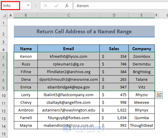
We want to find out the cell address of this named range.
So, let’s start the process like the one below.
📌 Steps:
- First of all, select. a cell and type the following formula into the selected cell.
=ADDRESS(ROW(Info),COLUMN(Info))

- Now, press ENTER, and all the cell addresses of the named range will appear.

If you run other versions of Excel than 365, then you have to use the following individual formula to get the first cell of the range, the last cell of the range, and the whole range.
- First Cell of the Range:
=ADDRESS(ROW(Info),COLUMN(Info))
- Last Cell of the Range:
=ADDRESS(ROW(Info)+ROW(Info)-1,COLUMN(Info)+COLUMN(Info)-1)
- The Whole Range:
=ADDRESS(ROW(Info),COLUMN(Info)&":"&ADDRESS(ROW(Info)+ROW(Info)-1,COLUMN(Info)+COLUMN(Info)-1)
5. Return Cell Address of Highest and Lowest Value
If you want to find out the cell address of the highest and the lowest cell values from a range of data, don’t worry. Excel allows a user to find out the highest and the lowest values from a range and also the cell addresses of the highest and the lowest values. For this purpose, we will have to apply the MAX, MIN, ADDRESS, MATCH, and COLUMN functions.
Now, proceed in the steps below.
📌 Steps:
- First of all, apply the MAX function to get the highest value from a data range.
=MAX(D5:D14)
Here, D5:D14 = lookup range
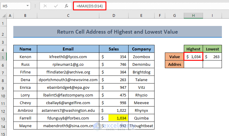
- Then, apply the MIN function to get the lowest value of the corresponding range.
=MIN(D5:D14)
Here,
- D5:D14 = lookup range

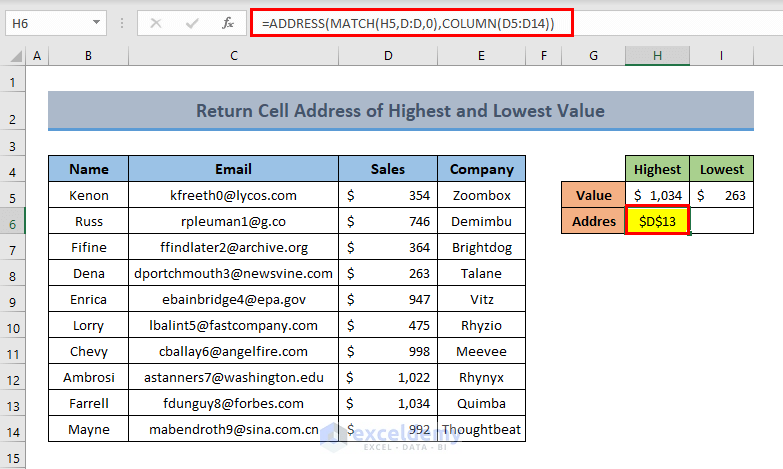
- After that, apply the following formula to get the cell address of the highest value. The MATCH function gives the row number and the COLUMN function gives the column number. Finally, the ADDRESS function returns the cell address.
=ADDRESS(MATCH(H5,D:D,0),COLUMN(D5:D14))
Here,
- H5 = the highest value
- Now, apply the following formula to get the cell address of the lowest value.
=ADDRESS(MATCH(I5,D:D,0),COLUMN(D5:D14))
Here,
- I5 = the lowest value
Read More: How to Return Cell Address of Match in Excel
Download Practice Workbook
You can download the practice book from the link below.
Conclusion
In this article, I have tried to show you some methods to return the cell address instead of the value in Excel. I hope this article has shed some light on your way to this. If you have better methods, questions, or feedback regarding this article, please don’t forget to share them in the comment box.
Related Articles
<< Go Back to Excel ADDRESS Function | Excel Functions | Learn Excel
Get FREE Advanced Excel Exercises with Solutions!
