Method 1 – Using a Combination of CELL, INDEX, and MATCH Functions
Steps
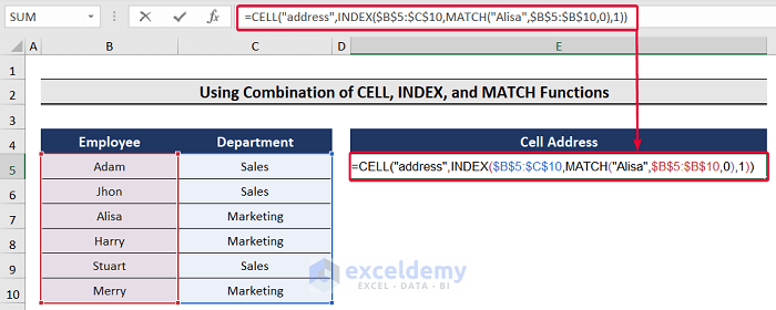
- Select cell E5.
- Enter the following formula:
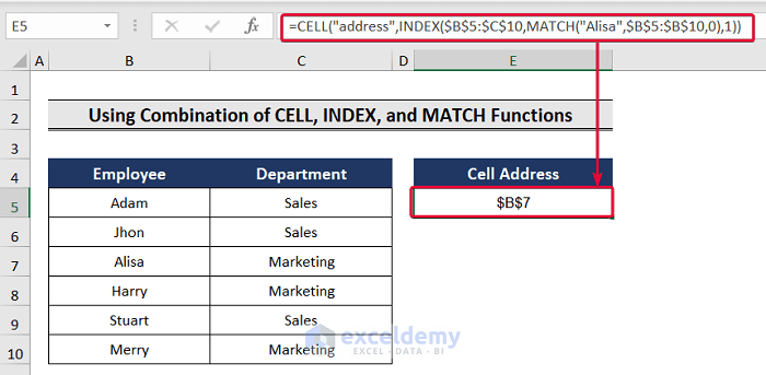
=CELL("address",INDEX($B$5:$C$10,MATCH("Alisa",$B$5:$B$10,0),1))- Press Enter.
- The result will be the cell address of the desired value (Alisa), which is B7.
Formula Break Down
- MATCH(“Alisa”,$B$5:$B$10,0): It looks for an exact match of the value Alisa in the lookup array B5:B10 and finds the value in row number 3.
- INDEX($B$5:$C$10,MATCH(“Alisa”,$B$5:$B$10,0),1): It returns the cell value at the intersection of row 3 and column 1. These numbers are rows and columns of the corresponding dataset. The output is Alisa.
- CELL(“address”,INDEX($B$5:$C$10,MATCH(“Alisa”,$B$5:$B$10,0),1)): It returns the address of Alisa, and it is B7.
Method 2 – Applying ADDRESS and MATCH Functions in Combination
Steps
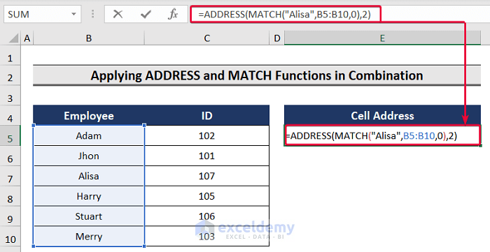
- Choose cell E5.
- Enter this formula:
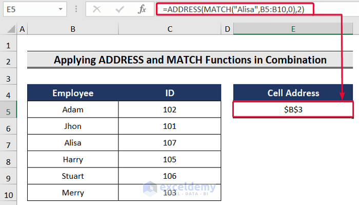
=ADDRESS(MATCH("Alisa",B5:B10,0),2)- Press Enter.
- The result will be the cell address containing the specific value (Alisa), which is $B$3.
Formula Break Down
- MATCH(“Alisa”, B5:B10,0): It looks for an exact match of the value Alisa in the lookup array B5:B10 and finds the value in row number 3.
- ADDRESS(MATCH(“Alisa”, B5:B10,0),2): It looks for the cell address of Alisa and it is in column 1, row number 3 of the array. So, the result is $B$3.
Read More: How to Use Cell Address in Excel Formula
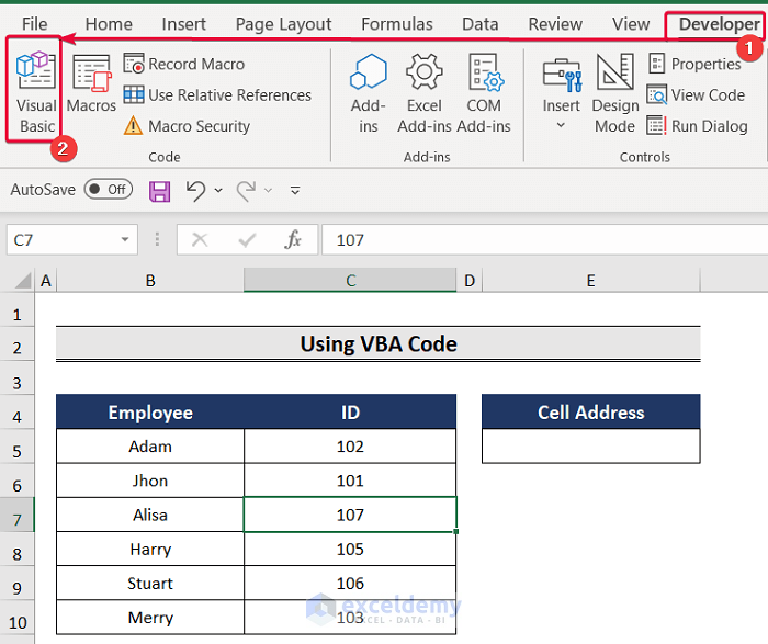
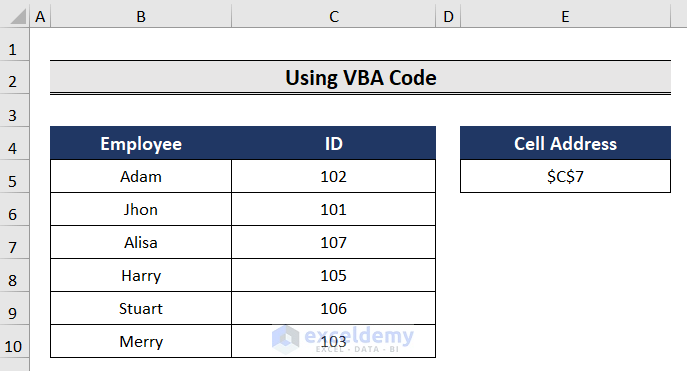
Method 3 – Using VBA Code
Steps
- Select any cell (e.g., C7) to find its address.
- Go to the Developer tab in the ribbon.
- Click on the Visual Basic tab.
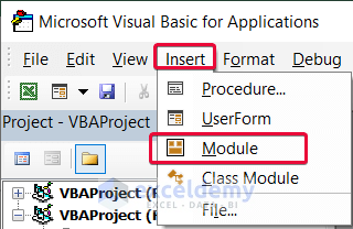
- Insert a new module.
- Enter the below code.
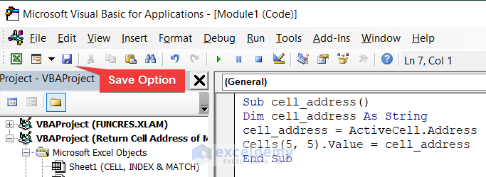
Sub cell_address()
Dim cell_address As String
cell_address = ActiveCell.Address
Cells(5, 5).Value = cell_address
End Sub- Save the code.
- Run the code.
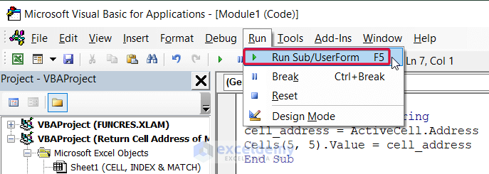
- The cell address will be displayed.
Read More: Excel VBA to Find Cell Address Based on Value
How to Return Cell Address Instead of Value in Excel
Steps
- In cell E5, enter this formula:
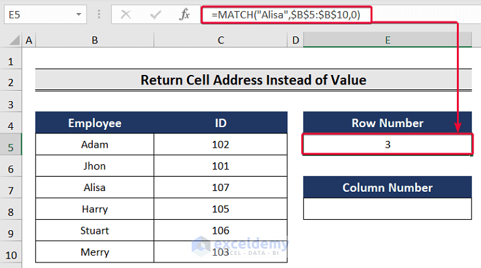
=MATCH("Alisa",$B$5:$B$10,0)- Press Enter.
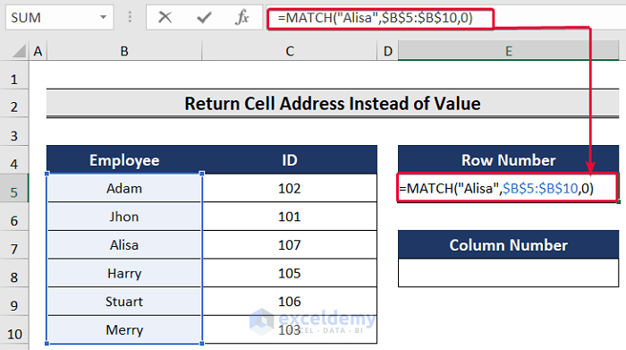
- This gives the row number of the cell containing the value.
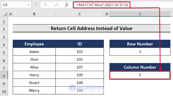
- For the column number, choose cell E8 and enter:
=MATCH("Alisa",$B$7:$C$7,0)- Press Enter.
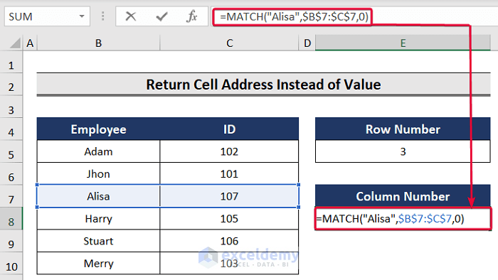
- The result will be the column number of the cell.
Download Practice Workbook
You can download the practice workbook from here:
Related Articles
<< Go Back to Excel ADDRESS Function | Excel Functions | Learn Excel
Get FREE Advanced Excel Exercises with Solutions!
