When working with Excel, it is a must to know clearly about cell addresses. Because, when you insert or extract formulas, the cells are the most important factor as they carry the values. In this article, I will demonstrate 5 ideal types of examples of cell addresses in Excel.
Example of Cell Address in Excel: 5 Conventional Cases
1. Cell Address with Relative Reference
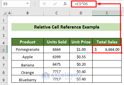
The most common example of a cell address in Excel is mainly of relative reference type. The example of relative reference is shown below.
📌 Steps:
- Say, you need to multiply cells C5 and D5.
- You can simply put an equal (=) sign and refer to the cells with an asterisk (*) symbol.
- Thus, the multiplication will take place automatically and here you addressed the cells with relative reference.
- For the other cells, you can simply drag your fill handle below to copy the same formula dynamically.
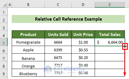
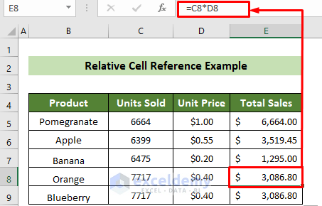
As a result, you can see all other multiplications are done for all the cells below. And, the cell addresses were changed automatically for all rows as the cells inside the formula were relative referenced cell addresses.
Read More: How to Use Cell Address in Excel Formula
2. Cell Address with Absolute Reference
Now, it might happen sometimes that you need an absolute cell-referenced address. That means, you will drag the fill handle but the cell reference won’t change. Go through the steps below to learn about the example of cell address of absolute reference type in Excel.
📌 Steps:
- To calculate commission, you need to multiply the total sales values with the commission rate.
- So, you can put the formula below in cell F5 and press the Enter key.
=E5*$H$5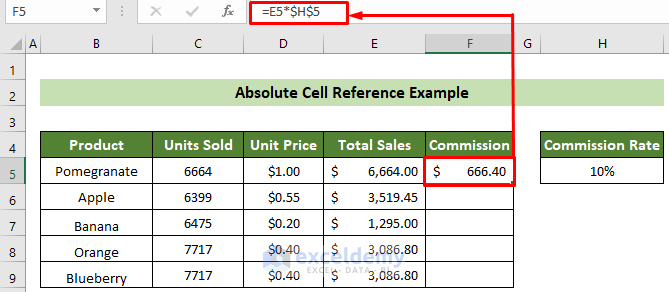
- Now, for other commissions, you can drag the fill handle below.
- You will see the formula is changing dynamically for E column cell addresses, but the H5 cell address is constant in every formula below.
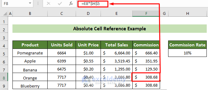
This happened because cell H5 is in the absolute reference address. You can make a cell absolute by putting a dollar ($) sign before the column and row number.
Read More: Excel VBA to Find Cell Address Based on Value
3. Cell Address with Mixed Reference
Now, you might need to use a cell address as a mixed cell reference. Say, you have a column with 3 values and a row with 3 values. Now, you need to multiply the values row-wise and column-wise individually. You can accomplish this with mixed cell reference by following the steps below.
📌 Steps:
- For the first result, click on cell C5 and insert the following formula.
=$B5*C$4- Subsequently, hit the Enter key.
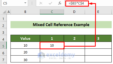
- Afterward, for all the other cells, drag your fill handle downward first and rightward next.
- Thus, you will get all the multiplication row-wise and column-wise.
- Here, the formulas changed dynamically, but only in one direction as you have used mixed cell reference.
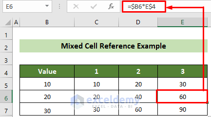
Here, to make the column absolute, you will need to put a dollar ($) sign before the column number, and to make the row absolute, you will need to put a dollar ($) sign before the row number.
4. Using Named Range as Cell Address in Excel
You can also use a named range to determine cell addresses in Excel. Say, you want to use a named range for the commission rate and calculate further. Go through the steps below to do this.
📌 Steps:
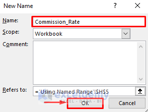
- First, click on cell H5 >> go to the Formula tab >> Define Names group >> Define Name tool.
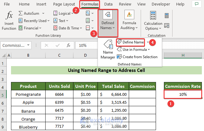
- As a result, the New Name window will appear.
- Following, at the Name: text box, write Commission_Rate and click on the OK button.
- At this time, for calculating commission, insert the following formula on cell F5.
=E5*Commission_Rate- Subsequently hit the Enter key.
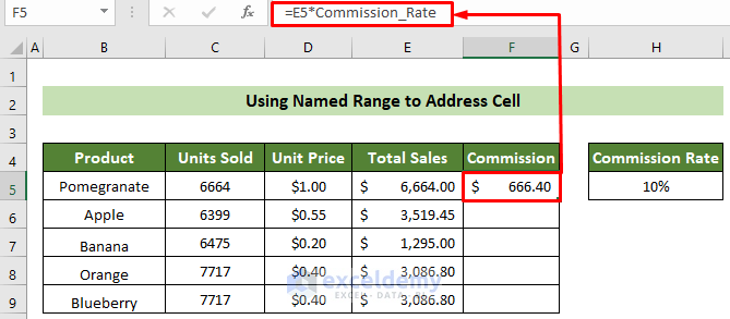
- As a result, you will get all the commissions for all sales values.
Here, for naming the H5 cell individually, the fill handle can not change this address in the formula dragging.
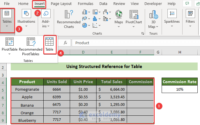
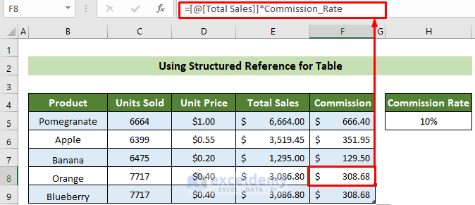
5. Using Structured Reference for Cells in an Excel Table Column
You can also use structured references for table column cells. Go through the steps below to learn this.
📌 Steps:
- At the very beginning, select your dataset.
- Following, go to the Insert tab >> Tables group >> Table tool.
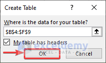
- As a result, the Create Table window will appear.
- Subsequently, click on the OK button with the default setup.
- At this time, click on cell F5.
- Subsequently, insert the following formula and press the Enter key.
=[@[Total Sales]]*Commission_Rate
- For all the other commission values, you can drag the fill handle below.
- It will dynamically change the formula with the table’s column with structured reference.
How to Switch Between Cell Reference Types in Excel
You can switch to different types of cell references by pressing the F4 key. Follow the guidelines below to do this properly.
- Press the F4 key once, if you want to make the cell absolute.
- Press the F4 key twice, if you want to make the cell mixed reference with an absolute row.
- Press the F4 key thrice, if you want to make the cell reference mixed with an absolute column.
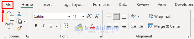
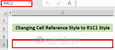
How to Change the Default Cell Reference/ Address Style to R1C1
By default, the cell reference style is to write the column heading first and then the row heading. You can change it to the R1C1 style by following the steps below.
📌 Steps:
- First and foremost, click on the File tab.
- Afterward, choose the Options option from the expanded File tab.
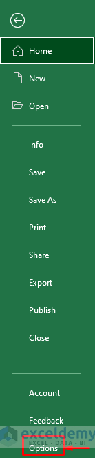
- As a result, the Excel Options window will appear.
- Subsequently, go to the Formulas tab >> tick the R1C1 reference style option and click on the OK button.
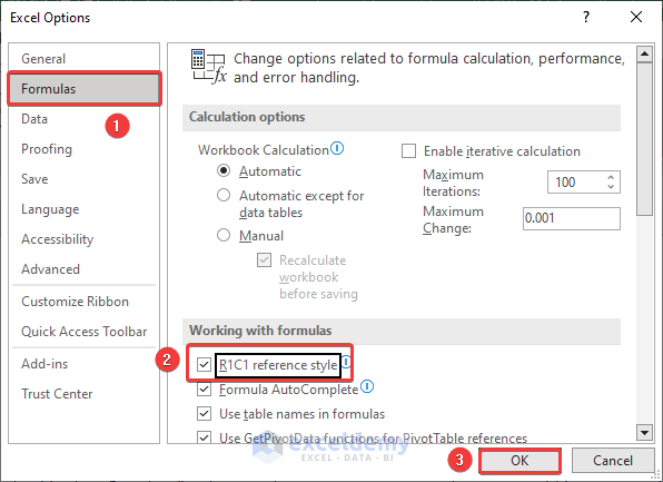
As a result, you will see every cell is now addressed as a row and column number.
How to Find Cell Address in Excel
Use ADDRESS Function:
Furthermore, you can use the ADDRESS function to find cell reference addresses in Excel. Go through the steps below to do this.
📌 Steps:
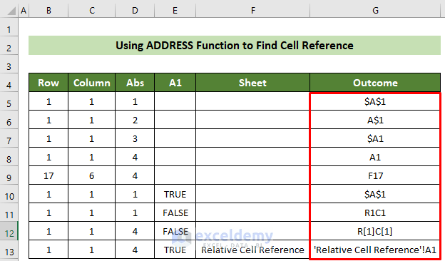
- At the very beginning, click on cell G5 and insert the following formula as per the values of the cells.
=ADDRESS(B5,C5,D5)- Subsequently, hit the Enter key.
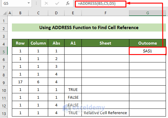
- Thus, you will see the cell address as per values.
- The ADDRESS function has five arguments. If you use all the arguments like the following formula, you will get the following result in cell G13.
=ADDRESS(B13,C13,D13,E13,F13)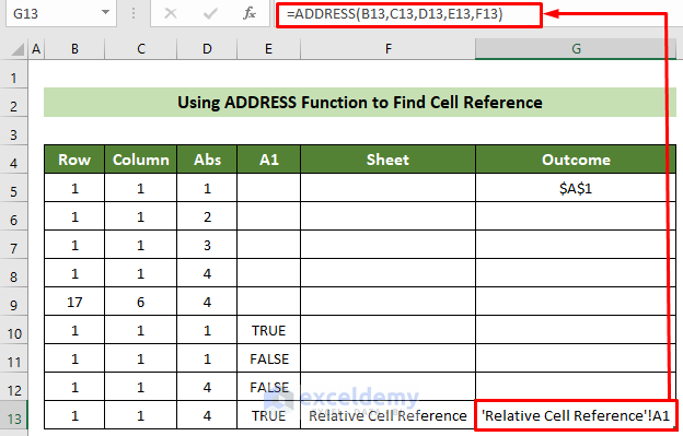
Thus, if you use the values according to the figure below in the ADDRESS function, you will get the result like the Outcome column cells.
Combine CELL, INDEX & MATCH Functions:
You can also combine the CELL, INDEX, and MATCH functions to find a cell address for definite values.
📌 Steps:
- To find the Banana value cell in the dataset, click on cell G5 first.
- Following, insert the formula below and press the Enter key.
=CELL("address", INDEX(B5:E9,MATCH("Banana",B5:B9,0),1))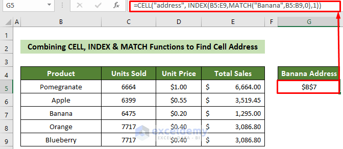
Thus, you will get the Banana cell address in cell G5.
Read More: How to Return Cell Address of Match in Excel
How to Create New Cell Address in Excel
Besides, you can combine the ADDRESS and MATCH functions to create a new cell address. Say, you want to find the Banana value in your dataset and create a new serial starting from our dataset.
📌 Steps:
- Initially, click on cell G5.
- Following, insert the formula below.
=ADDRESS(MATCH("Banana",B5:B9,0),2)- Subsequently, press the Enter key.
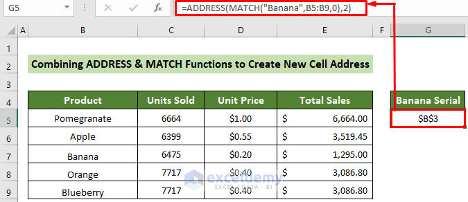
As a result, you will get the new serial of the Banana value starting from the dataset. As the Banana value is in column B and the third data of the dataset, the address would be $B$3.
Download Practice Workbook
You can download our practice workbook from here for free!
Conclusion
So, in this article, I have elaborately discussed the example of cell address in Excel and have shown you 5 ideal examples. Read the full article carefully and practice accordingly. I hope you find this article helpful and informative. You are very welcome to comment here if you have any further questions or recommendations.
Related Articles
- How to Get Cell Value by Address in Excel
- How to Copy Cell Address in Excel
- How to Return Cell Address Instead of Value in Excel
<< Go Back to Excel ADDRESS Function | Excel Functions | Learn Excel
Get FREE Advanced Excel Exercises with Solutions!
