Creating a named range in Excel is an easy task. But, if you want to make the named range dynamic so that whenever you add new data, the named range will update in a dynamic way, you have to do something more than just reference cells of the source data!
In this article, I will show you how to use the INDEX function of Excel to create a dynamic named range with detailed steps.
Steps to Create Dynamic Range Using Excel INDEX Function
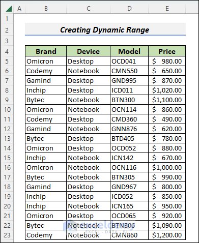
The following image shows the data with which we are going to demonstrate the procedures.
Step 1: Create an INDEX Formula with COUNTA and ROW Functions to Create a Dynamic Range
- We know that a range looks like this (A1:B10).
- Again, the INDEX function can be used as a cell reference.
- So, we will specify the first cell of the dynamic range and supply the second cell reference with the help of an INDEX formula.
- As a whole, the formula will be like the following.
=$C$5:INDEX($C:$C,COUNTA($C:$C)+ROW($C$4)-1)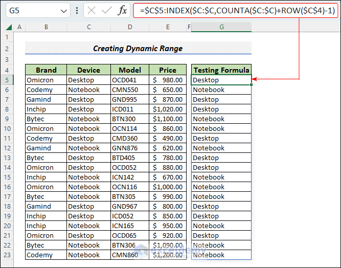
Formula Breakdown:
- We are going to create a dynamic range for the device names and hence use column C as the array of the INDEX function.
- The COUNTA function returns the number of non-blank cells in column C.
- But we need to reach the bottom of the data to get all the device names.
- So, we employ the ROW function, and it returns the row number of cell C4.
- The outputs of COUNTA and ROW together return the last row number of the data plus 1.
- So, you have to minus 1 and this will return C23 and the whole formula becomes C5:C23.
- Whenever you add another entry in column C, the row number of the INDEX function will increase by 1 (the COUNTA function is the main actor here) and will add the new item too, in the dynamic range.
- Test this by adding a new name in cell C24.
Step 2: Create a Named Range to Use the Dynamic Range Later in Any Formula
- We are done so far. To utilize the created dynamic range, we will now give a name to this range.
- To do that, select and copy the formula from cell G5.

- Now, go to the Formulas tab and click on the Define Name button.

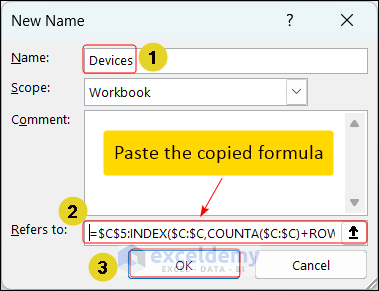
- The New Name window will appear.
- Give a suitable name to the range (Devices here).
- Paste the copied formula in the Refers to: box and press OK.
- You can also add any comment in the Comment box.
Step 3: Apply the Dynamic Named Range and Test If It Is Created Properly
- Finally, choose a suitable cell and write the following formula.
=Devices- After pressing Enter, you will immediately get the specified range.
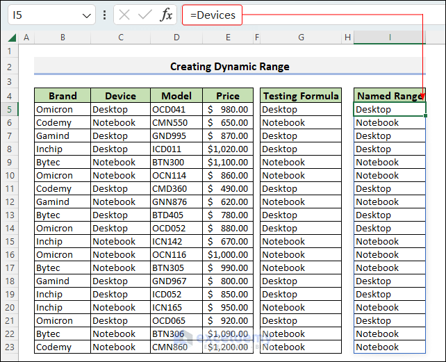
- Now, check if everything is working properly!

Note:
- You can also use the following formula to create the same dynamic range.
=FILTER(INDEX($B$5:$E$100,0, MATCH($C$4, $B$4:$E$4, 0)),$C$5:$C$100<>"")
- Here, we have utilized the MATCH function to supply the relevant row number of the INDEX function.
- The FILTER function is then used to handle the unnecessary zeros.
- We have given a new name Devices_MATCH to the new dynamic named range.

- To create a 2D dynamic range with the INDEX function, the following formula will go.
=$B$4:INDEX($1:$1048576,COUNTA($B:$B)+2,COUNTA($4:$4)+1)- This formula is similar to the main formula we have used here. The additional thing in this formula is- that we have supplied the column numbers too.
- We have added 2 with COUNTA($B:$B) because we have 2 blank cells in B1 and B3. If you wouldn’t count them, the formula couldn’t reach the bottom of the data.
- The same logic goes for adding 1 with COUNTA($4:$4).
- You cannot place this dynamic range in a cell that has row number 4, column B, or both. Because it will create a circular reference in that case and you will get a warning first and a 0 after pressing the OK button of the warning window.

Read More: Dynamic Named Range Based on Cell Value in Excel
Excel OFFSET Function: Alternative to INDEX to Create Dynamic Range
The OFFSET function is another option to create a dynamic range in Excel. If you feel better about working with the OFFSET function instead of INDEX, follow this workaround.
Steps:
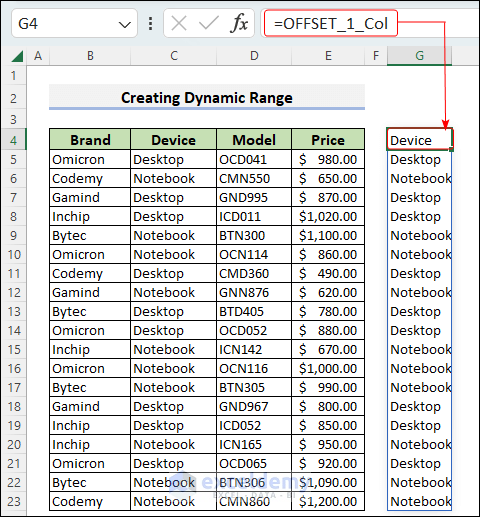
- To get 1 column (Device column) dynamic range, use the following formula.
=OFFSET($B$4,0,1,COUNTA($C:$C))- Here, the OFFSET function starts from cell B4 which is the starting cell of the data.
- Then we set the row number 0 and column number 1 since we want to remain in the same row of cell B4 but advance 1 column rightward.
- Then we specify the height of the output using the COUNTA function.
- Since there is no unnecessary data along column C, the COUNTA(C:C) formula will be enough here.
- To get multiple columns dynamic range (starts from cell B4, covers columns B to E, and so on), apply the following formula.
=OFFSET($B$4,0,0,COUNTA($B:$B)-1,COUNTA($4:$4))- Now, when you add any item in columns B and E, you will see the corresponding change in the dynamic range you have created.

Read More: OFFSET Function to Create & Use Dynamic Range in Excel
Quick Notes
- Use absolute reference when you create a named range. Otherwise, Excel will change the cell references in the formula and you will get a wrong output when you change the placement to another cell.
- In the Refers to: box, press the F2 key to make the right or left arrow keys work.
Download Practice Workbook
First, please download the following workbook for your practice.
Conclusion
So, we have shown how to create a dynamic range in Excel using the INDEX function. We have also covered the creation of 1D and 2D dynamic ranges and added the OFFSET alternative to the INDEX method. Feel free to share your thoughts with us.
Related Articles
- How to Create a Range of Numbers in Excel
- Create Dynamic Sum Range Based on Cell Value in Excel
- Data Validation Drop Down List with Excel Table Dynamic Range
<< Go Back to Dynamic Range | Named Range | Excel Formulas | Learn Excel
Get FREE Advanced Excel Exercises with Solutions!
