This is an overview:
The Excel OFFSET Function
- Objective:
Return a reference to a range that is a given number of rows and columns from a given reference.
- Syntax:
=OFFSET(reference, rows, cols, [height], [width])
- Arguments:
reference- A cell or a range of cells. Based on this reference, the offset parameters are applied.
rows- Row number that is counted downward or upward from the reference point.
cols- Column number that is counted to the right or to the left from the reference value.
[height]- Height or number of rows that will be returned as resultant values.
[width]- Width or number of the columns that will be returned as resultant values.
- Example:
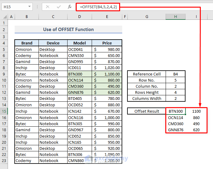
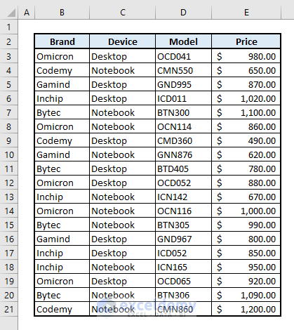
In the picture below, there are 4 columns with random names of computer brands, device types, model names and prices.
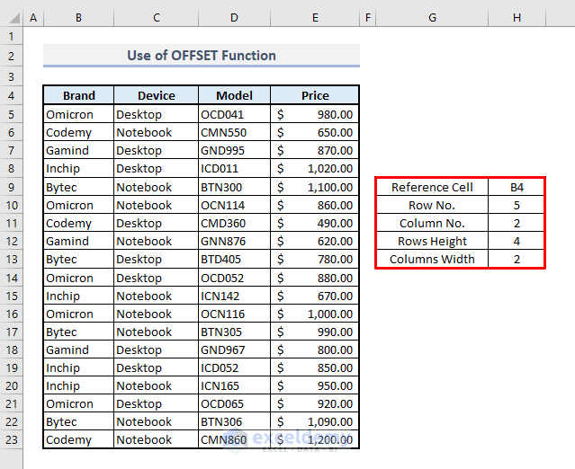
Use the arguments in Column H.
Steps:
- Enter the OFFSET function in H15:
=OFFSET(B4,5,2,4,2)- Press Enter.
An array of values will be returned based the selected arguments.

Formula Breakdown
the 1st argument is B4: a reference value. Going to the 5th row downward and 2nd column to the right of the reference cell, you’ll get D9. The row height is 2, so 4 cells to the bottom starting from D9 will be returned by the function. The column height- 2 means that 4 rows will expand to the next column to the right of Column D. The resultant array is D9:E12.
Read More: Dynamic Range for Multiple Columns with Excel OFFSET
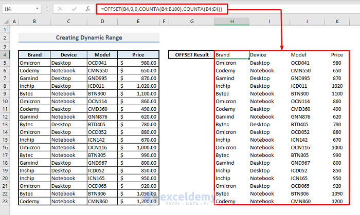
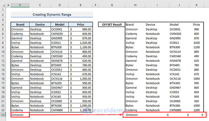
Example 1 – Creating a Dynamic Range with the OFFSET and the COUNTA Functions in Excel
Steps:
- Select H4 and enter the formula:
=OFFSET(B4,0,0,COUNTA(B4:B100),COUNTA(B4:E4))- Press Enter.
This is the output.
Formula Breakdown
In the argument section, row height is assigned to COUNTA(B4:B100) (rows up to the 100th row in the spreadsheet, so that new values are stored to the 100th row). The column width is defined as COUNTA(B4:E4), columns (B, C, D, E) are assigned to the function based on the reference value selected in the OFFSET function.
If you enter a value, the resultant value will be displayed in the OFFSET table.
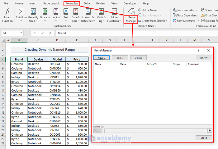
Example 2 – Using the Name Manager to Create a Dynamic Named Range with the OFFSET and the COUNTA Functions
Step 1:
- In the Formulas tab, select Name Manager.
- Select New to open the Name Editor box.
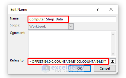
Step 2:
- Name the dataset or the range of cells you want to offset.
- In the reference box, enter the formula:
=OFFSET(B4,0,0,COUNTA(B4:B100),COUNTA(B4:E4))- Click OK.
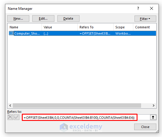
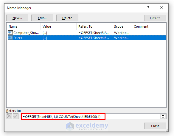
The defined name will be displayed with the reference formula.
Step 3:
- Close the Name Manager and go back to your spreadsheet.
Step 4:
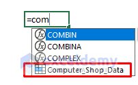
- Select any cell in your spreadsheet and start entering the defined name. You’ll find the defined name in the function list.
- Select that function.
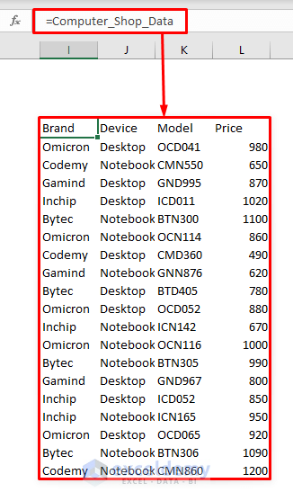
- Press Enter.
You’ll see the resultant array:
Read More: Dynamic Named Range Based on Cell Value in Excel
Example 3 – Using a Dynamic Named Range for Calculations
Step 1:
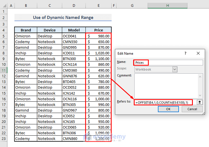
- Open the Name Editor and name the range: Prices.
- In the reference box, enter the formula:
=OFFSET(E4,1,0,COUNTA(E5:E100),1)- Click OK.
Prices will be displayed with a reference formula.
Step 2:
- Close the Name Manager and go back to your spreadsheet.
Step 3:
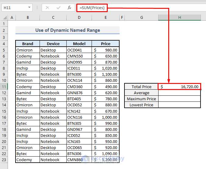
- Select H11 and enter the formula:
=SUM(Prices)- Press Enter.
You’ll get the total prices of all devices.
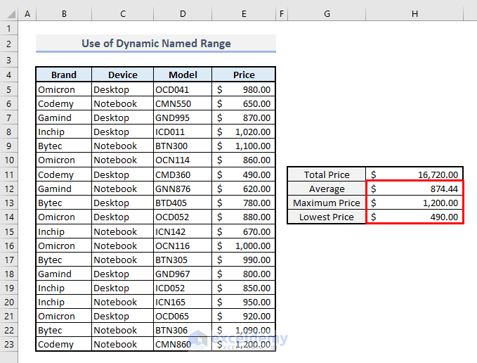
Using the AVERAGE, MAX & MIN functions, you can evaluate other data in Column H:
Read More: Create Dynamic Sum Range Based on Cell Value in Excel
An Alternative to the OFFSET: Creating a Dynamic Range with the INDEX Function
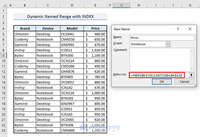
Step 1:
- Open the Name Editor and enter the formula in the reference box:
=INDEX(B5:E100, 0, MATCH(E4, B4:E4, 0))- Press Enter.
This is the output.
Step 2:
- Close the Name Manager.
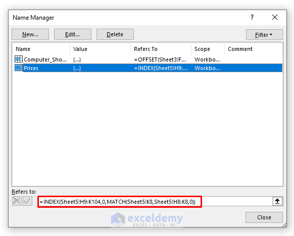
You can use the dynamic named range in your spreadsheet.
Read More: How to Create Dynamic Range Using Excel INDEX Function
Download Practice Workbook
Download the Excel workbook.
Related Articles
- How to Create a Range of Numbers in Excel
- Data Validation Drop Down List with Excel Table Dynamic Range
<< Go Back to Dynamic Range | Named Range | Excel Formulas | Learn Excel
Get FREE Advanced Excel Exercises with Solutions!
