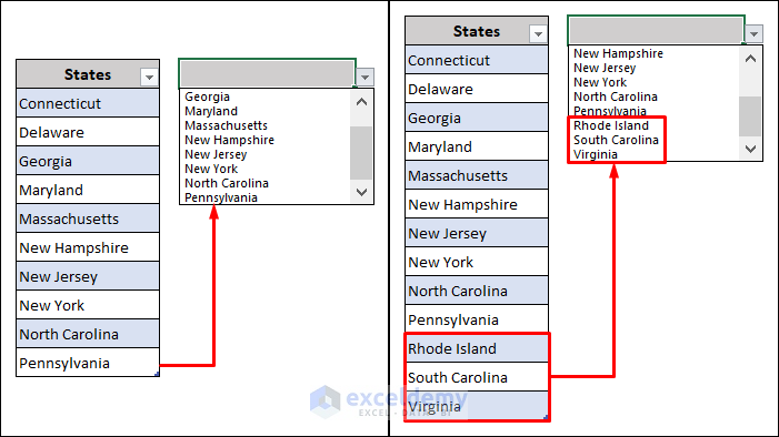
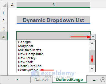
This article illustrates how to create a data validation drop down list with an Excel table dynamic range. This will save you a lot of time and energy. The following picture highlights the purpose of this article. Have a quick look through to see how to do that.
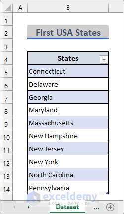
We will use the following Excel Table to highlight the methods. The table contains a list of names of some of the 13 original states of the USA. So let’s begin.
1. Using Defined Range for Data Validation Drop Down List with Excel Table Dynamic Range
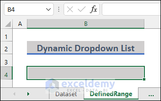
Imagine you want to create the dynamic dropdown list in cell B4 in the DefinedRange worksheet. Then follow the steps below to be able to do that by creating a defined range.
📌 Steps
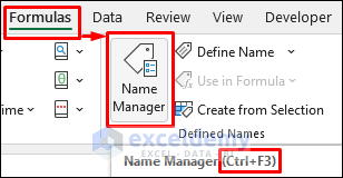
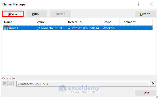
- First, you need to select Formulas >> Name Manager to open the Name Manager window. You can use the CTRL+F3 shortcut to do that too.
- Then select New on the Name Manager window.
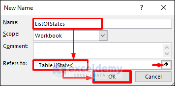
- Next, change the name to ListOfStates in the New Name dialog box. After that, enter the following formula in the Refers to: field. Then hit the OK button.
=Table1[States]- Here Table1 is the name of the dataset table. And States refers to the header of the table.
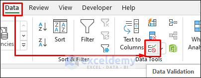
- Now select cell B4 and then select Data >> Data Validation as shown in the following picture.
- Next, go to the Settings tab in the Data Validation After that, choose List as the Validation criteria using the dropdown arrow.
- Then, enter the following formula in the Source field and hit the OK You can also click on the Source field and then press F3 to do that.
=ListOfStates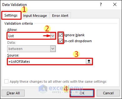
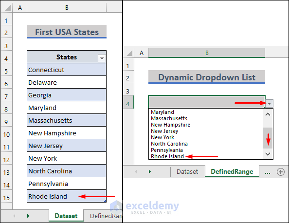
- After that, you will see the dropdown list working as shown below.
- Now enter values in the adjacent cells below the table. After that, you will see the dropdown list to change accordingly.
2. Inserting INDIRECT Function to Make Data Validation Drop Down List with Excel Table
You can also create a dynamic dropdown list with the INDIRECT function. Applying the following steps will be sufficient for that.
📌 Steps
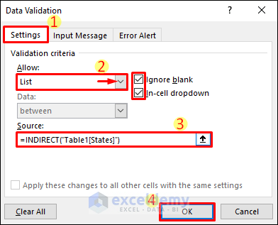
- First, select cell B4 in the INDIRECT worksheet. Then select Data >> Data Validation as in the earlier method.
- Next, set the Validation criteria to List. After that, enter the following formula in the Source field and then hit the OK button.
=INDIRECT("Table1[States]")- Here Table1 is the name of the dataset table. And States refers to the header of the table.
- Then you will see the dropdown list working as follows.
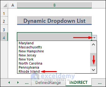
- Now, enter values in the adjacent cells below the table to verify if the dropdown list is dynamic or not. Then you will see the dropdown list changing accordingly.

3. Applying OFFSET Function for Data Validation Drop Down List with Excel Table Dynamic Range
You can also use the OFFSET function to create a dynamic dropdown list with an Excel table. Follow the steps below to do that.
📌 Steps
- First, select cell B4 in the worksheet named OFFSET. Then select Data >> Data Validation as in the earlier methods.
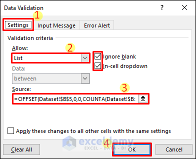
- Now, choose List as Validation criteria from the Data Validation window.
- After that, enter the following formula in the Source field and then hit the OK button.
=OFFSET(Dataset!$B$5,0,0,COUNTA(Dataset!$B:$B)-2,1)- The COUNTA function in the formula counts cells in a range excluding blank cells. -2 in the formula is used for the 2 cells (B2, B4) in the dataset which do not contain the actual data we want in the dropdown list.
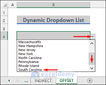
- Then you will see the dropdown list working as follows like in the earlier methods.
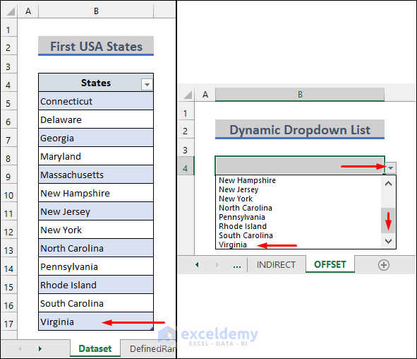
- Now enter new values again in the adjacent cells below the table. After that, the dropdown list will be updated automatically.
Read More: OFFSET Function to Create & Use Dynamic Range in Excel
Things to Remember
- The methods do not work properly if any cells in the table are blank. You can delete the rows containing the blank cells instead.
- Do not change the table name after applying the second method.
Download Practice Workbook
You can download the practice workbook from the download button below.
Conclusion
Now you know how to create a data validation dropdown list with an Excel table dynamic range. Please let us know if this article has solved your problem. You can use the comment section below for further queries or suggestions.
Stay with us and keep learning.
Related Articles
- Create Dynamic Sum Range Based on Cell Value in Excel
- How to Create a Range of Numbers in Excel
- Dynamic Range for Multiple Columns with Excel OFFSET
- Dynamic Named Range Based on Cell Value in Excel
- How to Create Dynamic Range Using Excel INDEX Function
<< Go Back to Dynamic Range | Named Range | Excel Formulas | Learn Excel
Get FREE Advanced Excel Exercises with Solutions!
