Dynamic Sum Range Based on Cell Value in Excel: 4 Ways to Create

Written by Mursalin Ibne Salehin

Last updated: Apr 16, 2024

Method 1 – Use INDEX Function to Create Dynamic Sum Range Based on Cell Value in Excel

We will use a dataset that contains information about the Sales Amount of the first two months of some Sellers.

STEPS:

Create a new column for the row numbers in Column C and a new row for column numbers in Row 6.

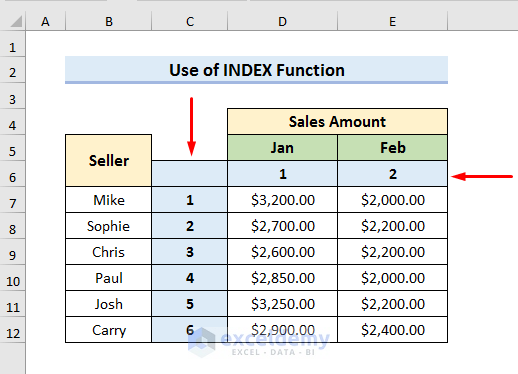
In this case, it means Row 7 of the sheet is the first row and Column D is the first column of our array (D7:E12).
Write Rows, Columns, and Sum in Cell G5 to G7 like the picture below.
Type the row and column numbers in cells H5 and H6.

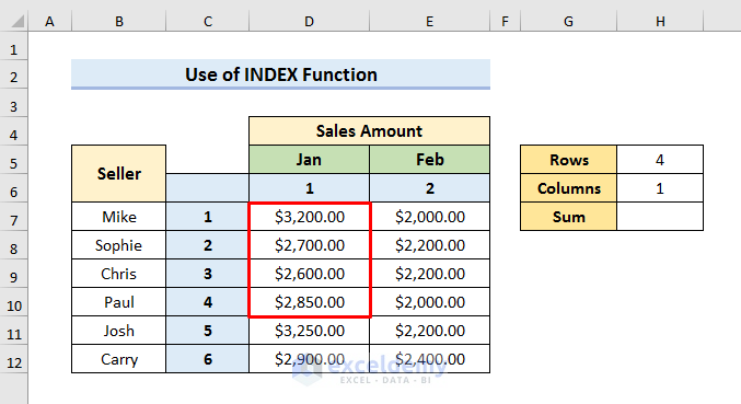
Rows = 4 and Columns = 1 denote the values Cell D7 to D10.
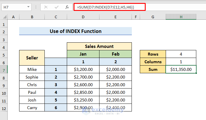
Select Cell H7 and type the formula:

=SUM(D7:INDEX(D7:E12,H5,H6))

Hit Enter to see the result in Cell H7.

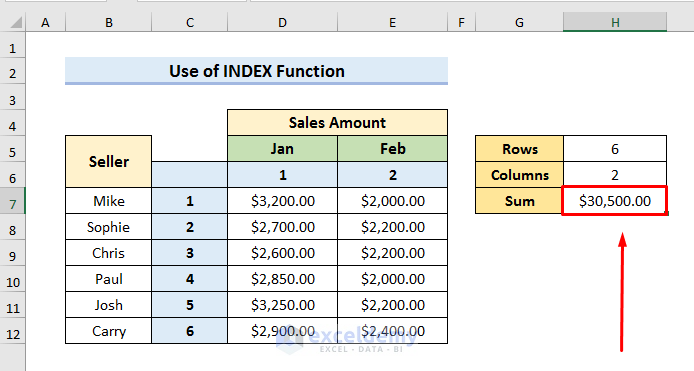
If we change the values of Rows and Columns, the Sum will be dynamically updated.

How Does the Formula Work?

INDEX(D7:E12,H5,H6)

The INDEX Function returns a value or reference of the cell at the intersection of a particular row and column in a given range. We have used the INDEX Function to get the last cell. Here, the first argument is the array(D7:E12). The second argument (H5) denotes the rows and the third argument (H6) denotes the columns of the array.

SUM(D7:INDEX(D7:E12,H5,H6))

The Sum Function is just summing up the values starting from D7. We used the INDEX Function to reference the last cell of the selected range.

When simplified, the formula becomes:

=SUM(first cell:INDEX(array,rows,columns))

Method 2 – Apply OFFSET Function to Define Dynamic Sum Range Based on Cell Value

Let’s use the same dataset as in the previous method.

STEPS:

Select Cell G7.
Copy this formula:

=SUM(OFFSET(C6,0,0,G5,G6))

Hit Enter to see the result in Cell G7.

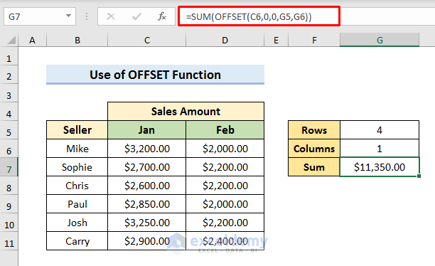
Here, the OFFSET Function returns a range that starts from Cell C6. Cell G5 and G6 define the height and width of the range.

If we change the values of Cell G5 and G6, the Sum will be automatically updated.

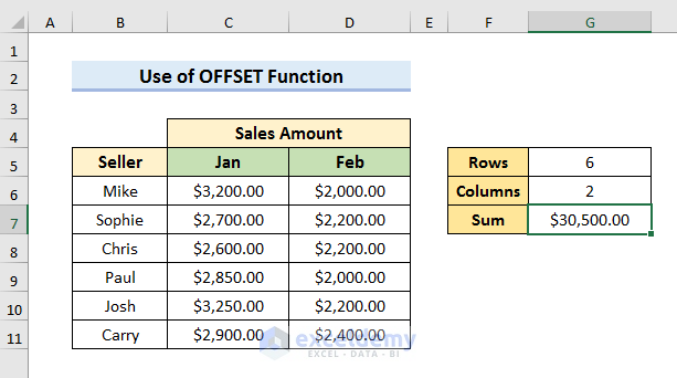
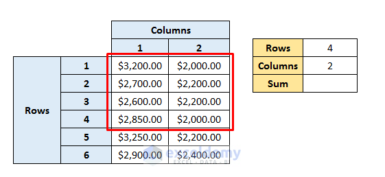
Here, Rows = 4 and Columns = 2 indicate the highlighted values of the range.

Method 3 – Excel Dynamic Sum Range Based on Cell Value with MATCH Function

Here, we will use the same dataset but exclude the sales amount of February month.

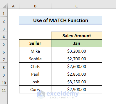
STEPS:

Create cells to write the seller’s name and the Sum. We have created these cells in Column E.

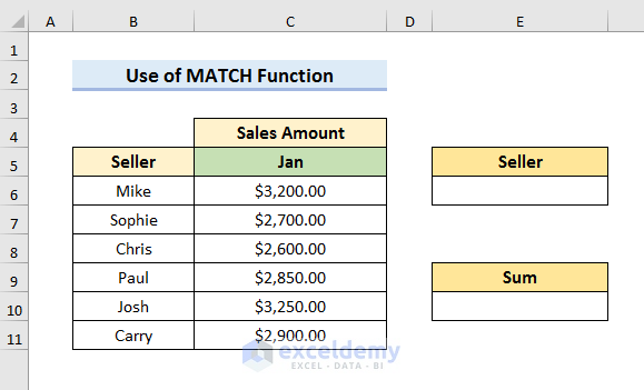
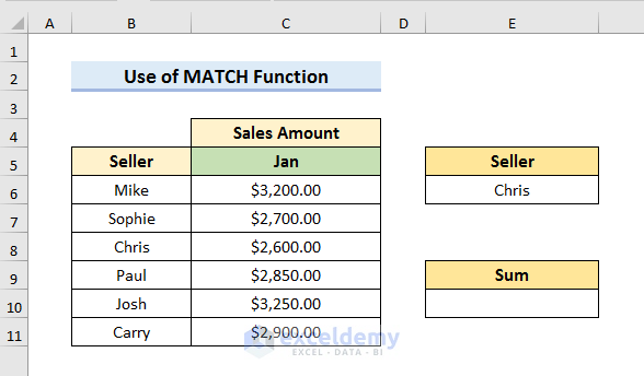
Write a seller’s name in Cell E6. We have written Chris.

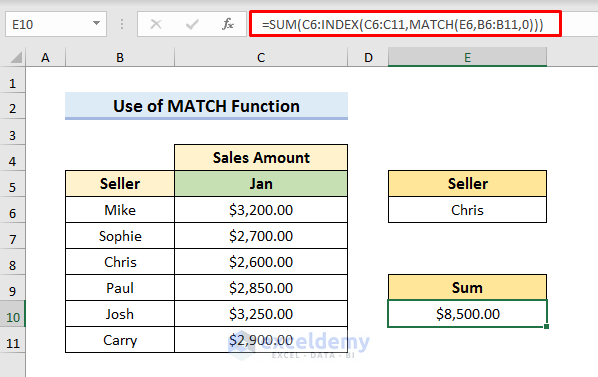
Select Cell E10 and type the formula:

=SUM(C6:INDEX(C6:C11,MATCH(E6,B6:B11,0)))

Press Enter to see the result.

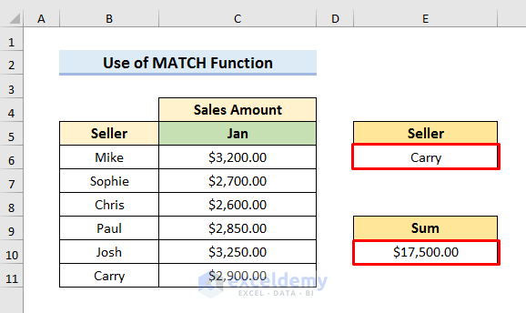
If we change the name of the seller, the Sum will be dynamically updated.

How Does the Formula Work?

MATCH(E6,B6:B11,0)

The MATCH Function finds the position of the selected seller in the range of the sellers.

INDEX(C6:C11,MATCH(E6,B6:B11,0))

The INDEX Function returns a value from the range C6:C11. The second argument of the INDEX Function is the position of the element that we need to return.

SUM(C6:INDEX(C6:C11,MATCH(E6,B6:B11,0)))

If we put the previous INDEX Function formula inside the SUM Function, the INDEX Function will return the reference of the cell and then, sum it up.

Method 4 – Create Dynamic Sum Range Based on Another Cell Value in Excel

We will use the previous dataset for this method.

4.1 Insert INDIRECT & CONCATENATE Functions Together

STEPS:

Create the dataset structure like the picture below.

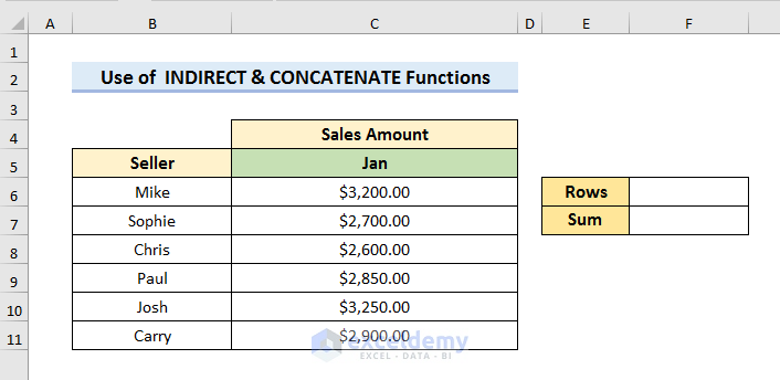
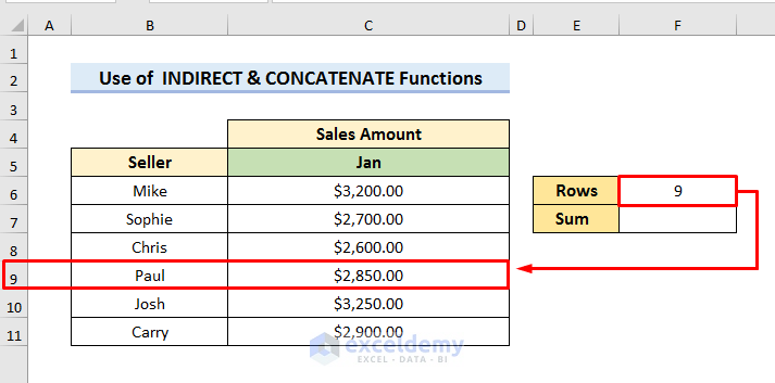
Here, 9 in Cell F6 refers to ROW 9 of the sheet.

Select Cell F7 and type the formula:

=SUM(C6:INDIRECT(CONCATENATE("C",F6)))

Hit Enter to see the result.

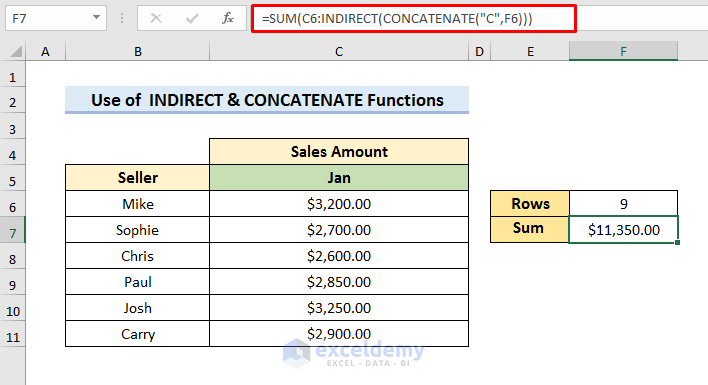
Here, C6 is the first cell of the column that we need to sum, Column C is the column where we need to perform the sum operation, and we sum up based on Cell F6. The INDIRECT(CONCATENATE(“C”,F6) part of the formula returns the cell reference for the end of the sum array, combining C with the number in the F6 cell.

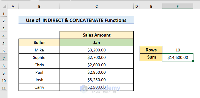
If we change the value of Cell F6, the result is automatically updated.

If you want to sum two columns, use the below formula:

=SUM(C6:INDIRECT(CONCATENATE("C",F6)),D6:INDIRECT(CONCATENATE("D",F6)))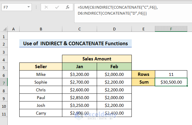

How Does the Formula Work?

C6:INDIRECT(CONCATENATE(“C”,F6))

This is the first argument of the SUM Function. It refers to the range of Column C that we want to sum.

D6:INDIRECT(CONCATENATE(“D”,F6))

Here, it is the second argument of the SUM Function. It refers to the range of Column D that we need to sum.

SUM(C6:INDIRECT(CONCATENATE(“C”,F6)),D6:INDIRECT(CONCATENATE(“D”,F6)))

Now, the SUM Function is just summing up the ranges of Column C and D.

4.2 Use INDIRECT Function Only

INDIRECT can also be used to return a range, and it already accepts string values.

STEPS:

Create the dataset structure like the picture below.

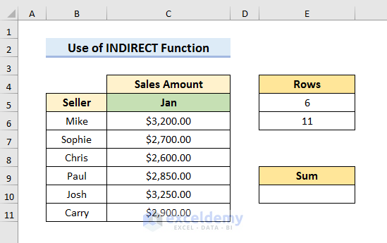
This will sum the values of Row 6 to Row 11 of Column C.
Select Cell E10 and type the formula:

=SUM(INDIRECT("C" &E5& ":C" &E6))

Hit Enter to see the result.

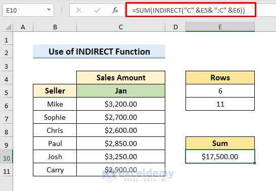
Here, we have used the INDIRECT Function to create the variable range of cell references that we want to sum. Then, we have embedded it inside the SUM Function.

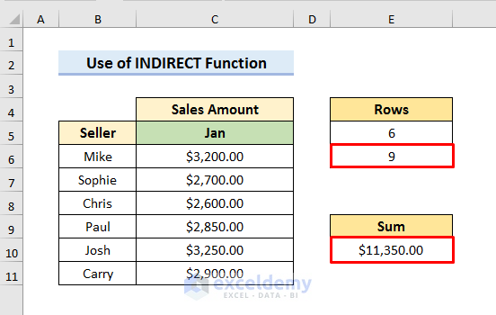
If we change the value of Cell E6, the Sum will automatically be updated.

Download Practice Book

Download the practice book here.

Dynamic Sum Range Based on Cell Value.xlsx

<< Go Back to Dynamic Range | Named Range | Excel Formulas | Learn Excel

Get FREE Advanced Excel Exercises with Solutions!

Sub inventory_check() Set Rng = Selection Prev_bal = InputBox("Insert Previous Balance") Sum = 0 Count = 0 Rng.Cells.Interior.ColorIndex = xlNone For i = 1 To Rng.Rows.Count Sum = Sum + Rng.Cells(i, 1) If Sum > Int(Prev_bal) Then Rng.Cells(i, 1).Interior.Color = VBA.RGB(249, 176, 103) Count = Count + 1 If Count > 0 Then Exit Sub End If End If Next i End Sub

9 Comments

Uday Kumar Feb 13, 2023 at 10:05 PM

I am using this formula in conditional formatting in office 2019 version
=SUM(B$3:INDEX(B$3:B3,ROWS(B$3:B3)-1))<=B$35
but it throws error like "You may not use reference operators (such as union, intersection and ranges) or array constants for conditional formatting criteria"

However the same formula works fine in 2007 version of excel. Even in 2019 version, when i write the same formula in excel it works, but not in conditional formatting..

plz help
- Reply
  Sabrina Ayon Feb 14, 2023 at 1:00 PM
  
  Hello, UDAY KUMAR!
  It seems that the error message you received is related to the use of reference operators in the formula.
  The formula you were using in the conditional formatting rule contains a reference operator and the INDEX function, which can be interpreted as an array constant. The error message you received indicates that the use of such operators and array constants is not allowed in conditional formatting criteria.
  
  To avoid using the reference operator and array constant, you can use the INDIRECT function. Here’s an example formula that uses the INDIRECT function:
  
  =SUM(INDIRECT("B$3:B" & ROW()))<=$B$35
  
  The INDIRECT function takes a text string argument that specifies a cell reference and returns the value of the cell. By concatenating the starting and ending cell references with the ROW function, we can create a dynamic reference to the range we want to sum.
  
  Hope this will help you. If not, can you please send me your excel file via email? ([email protected]).
  Good Luck!
  
  Regards,
  Sabrina Ayon
  Author, ExcelDemy.
  - Reply
    Uday Kumar Feb 18, 2023 at 6:19 PM
    
    Hello Sabrina Ayon
    Thanks for replying. I tried ur solution but it did not help. I have sent u test file with complete problem on ur gmail ID. plz respond.
    Thank you.
    Uday Kumar
    - Zahid Hasan Feb 20, 2023 at 4:07 PM
      
      Dear Uday Kumar,
      Good afternoon! First of all, thank you for the detailed description of the problem. What I have understood from your email, is that you want to highlight the cell where the sum of the distributed X items crosses the Previous Balance.
      Using the Excel formula in this situation becomes quite complicated and returns errors when used in the Conditional Formatting option. But running a simple Macro can achieve your desired output without any hassle.
      If you don’t know how to run a Macro, don’t worry. It’s not that complicated at all. Just follow the steps below, and you will be good to go.
      Step 01: Create a Blank Module
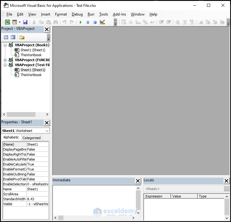
      At first, you will need to create a blank Module. The Module is where we will write the code. Simply press ALT + F11 on your keyboard to open the following window on your worksheet.
      
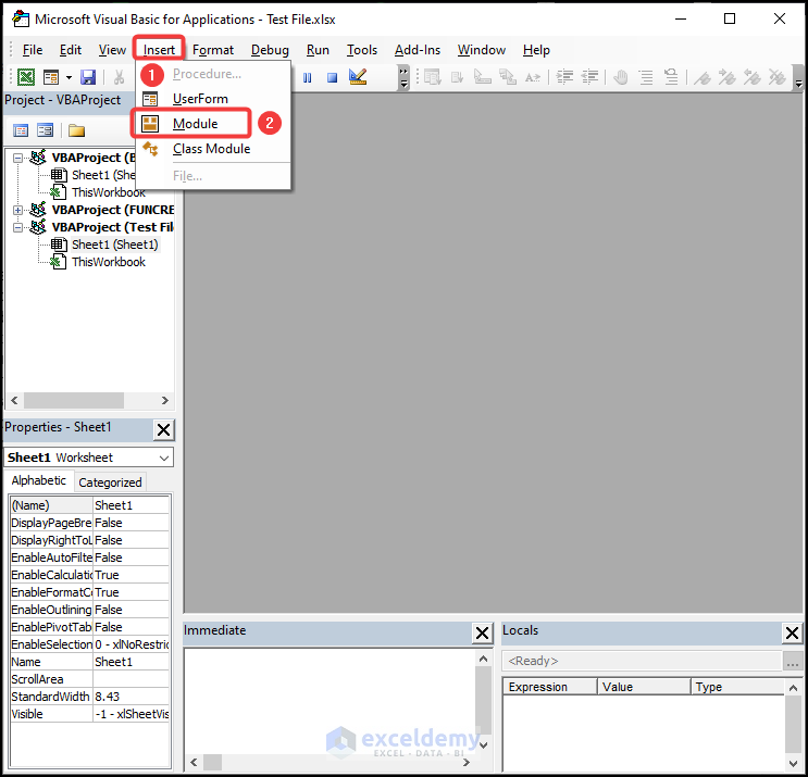
      Now, go to the Insert tab and choose the Module option from the drop-down list.
      
      Step 02: Write and Run VBA Code
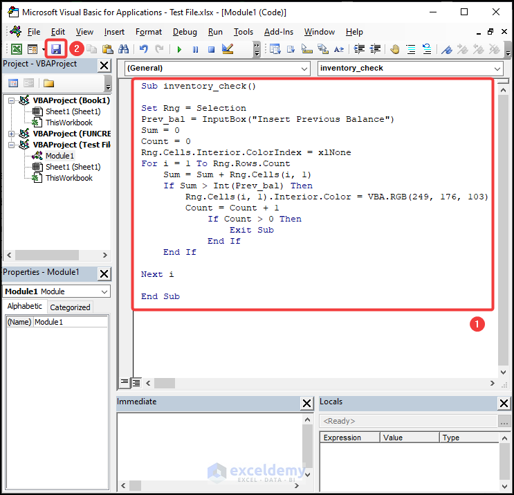
      Now, a blank Module will be created.
      Then, copy the following code and paste it into the blank Module.
      
      Sub inventory_check() Set Rng = Selection Prev_bal = InputBox("Insert Previous Balance") Sum = 0 Count = 0 Rng.Cells.Interior.ColorIndex = xlNone For i = 1 To Rng.Rows.Count Sum = Sum + Rng.Cells(i, 1) If Sum > Int(Prev_bal) Then Rng.Cells(i, 1).Interior.Color = VBA.RGB(249, 176, 103) Count = Count + 1 If Count > 0 Then Exit Sub End If End If Next i End Sub
      
      After that, click on the Save icon.
      
      Following that, close the VBA window or simply press ALT + F11. This will take you back to your worksheet.
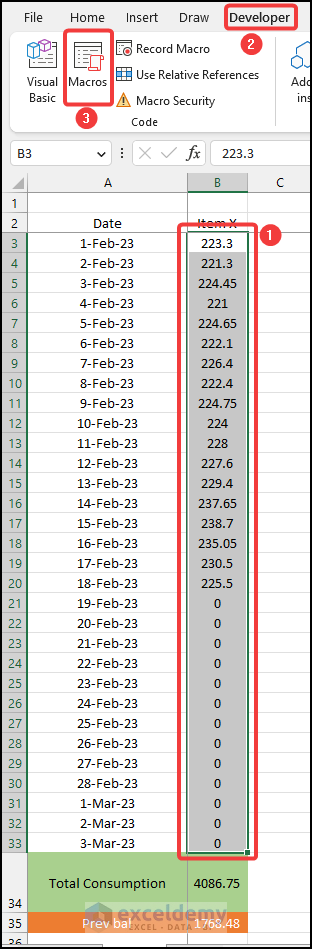
      Now, carefully select the range of data.
      Then, go to the Developer tab and click on the Macros option.
      
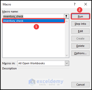
      Subsequently, the Macro dialogue box will open.
      Now, select the inventory_check option and click on Run.
      
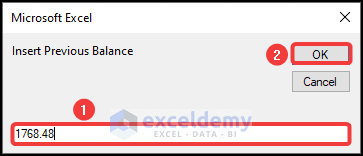
      Then a window will appear asking you for the Previous Balance. You need to enter the previous balance here and then click OK.
      
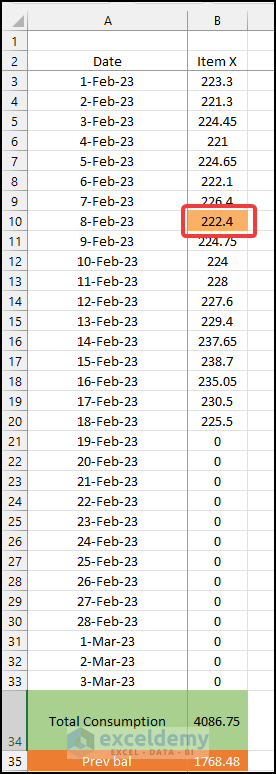
      Boom! The highlighted cell will indicate your desired output.
      You can change the Previous Balance according to your need and the highlighted cell will be changed accordingly.
      
      Things to Remember
      If you don’t have the Developer option enabled then follow this article to enable it.
      Don’t forget to save the file as Macro Enabled Workbook.
      I sincerely hope that this solves the issue you are facing. If any part of the solution is unclear to you, please let us know.
      
      Regards
      Zahid Hasan
      ExcelDemy
Uday Kumar Feb 21, 2023 at 11:38 AM

Thanks Hassan for the Help..
There are certain reasons I do not want to use Macro, though I know how to use it. Secondly, as u can see in the test file sent to u in email, formula gives perfectly fine result in google spreadsheet, in excel cell but not in the conditional formatting area. So, I do not know what is going wrong. Do u have any opinion about that ??
- Reply
  Zahid Hasan Feb 22, 2023 at 11:15 AM
  
  Dear Uday Kumar,
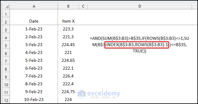
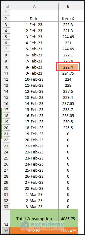
  Good day! I can comprehend how upsetting this situation could be. It took me a while to understand it, too. Hence, the portion of your formula that I have highlighted in the following figure is essentially what is causing the issue when doing Conditional Formatting.
  
  It will display an error in the Conditional Formatting when you specify a range using both a cell reference and a formula. As the goal of this formula is to add up to the cell that comes before the active cell, you can use the following formula instead. Here I simply replaced INDEX(B$3:B3,ROWS(B$3:B3)-1) by B2. The complete formula is:
  =AND(SUM(B$3:B3)>B$35, IF(ROWS(B$3:B3)<>1, SUM(B2:B$3)<=B$35, TRUE))
  Just paste this formula in the Conditional Formatting option and you will have your desired output as shown below.
  
  That should take care of your problem, I hope. If you run into any problems, please let us know.
  
  Regards
  Zahid Hasan
  ExcelDemy
Uday Kumar Feb 24, 2023 at 6:53 PM

Hello Zahid Hasan,
Can u plz suggest a non macro method for a solution to above problems…actually there are certain reasons that I do not want to use it.
- Reply
  Shamima Sultana Feb 26, 2023 at 9:47 AM
  
  Hello Uday Kumar,
  
  Kindly check the reply to your previous comment. We have given you a non-macro solution.
Uday Kumar Mar 4, 2023 at 8:49 PM

Thanks Sabrina Ayon, Hassan, Shamima Sultana for providing an intelligent solution by getting around the problem. It worked !

But for the sake of learning, compatibility issue between 2007 and 2019 remains to be quite baffling in current situation with the latest version not behaving properly. Its behaviour started appearing to me more as a magical problem than as a logical problem.

But any way thanks to the team!!

Dynamic Sum Range Based on Cell Value in Excel: 4 Ways to Create

Method 1 – Use INDEX Function to Create Dynamic Sum Range Based on Cell Value in Excel

Method 2 – Apply OFFSET Function to Define Dynamic Sum Range Based on Cell Value

Method 3 – Excel Dynamic Sum Range Based on Cell Value with MATCH Function

Method 4 – Create Dynamic Sum Range Based on Another Cell Value in Excel

4.1 Insert INDIRECT & CONCATENATE Functions Together

4.2 Use INDIRECT Function Only

Related Articles

Leave a reply Cancel reply