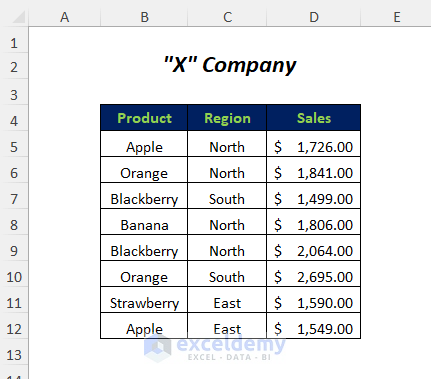
We have a dataset of a company to demonstrate the ways of using a dynamic range in VBA.
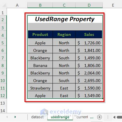
Method 1 – Select Cells Containing Values Through UsedRange Property
Steps:
- Go to Developer Tab>>Visual Basic Option.
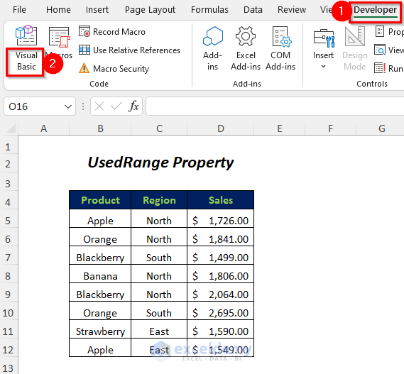
- The Visual Basic Editor will open up.
- Go to Insert Tab >> Module Option.
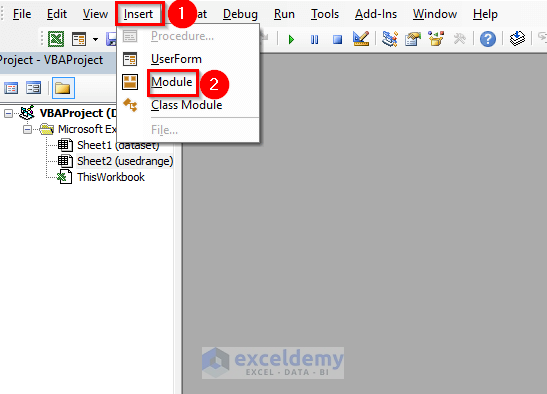
- Enter the following code:
Sub dynrange1()
Worksheets("usedrange").UsedRange.Select
End Sub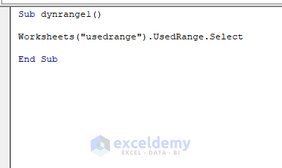
Note:
Here, “usedrange” is the sheet name. UsedRange property will select all the cells in this worksheet that have values in them.
- Press F5.
- Select the whole data range, including the heading.
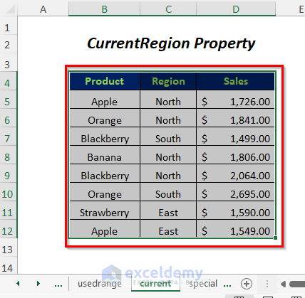
Method 2 – Choose Dynamic Range Including Headers with CurrentRegion Property
Steps:
- Follow the Steps of Method 1.
- Enter the following code:
Sub dynrange2()
Dim sht As Worksheet
Dim firstCell As Range
Set sht = Worksheets("current")
Set firstCell = Range("B5")
firstCell.CurrentRegion.Select
End Sub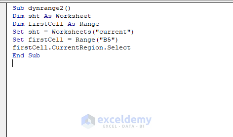
Note:
- Here, sht, firstCell are declared as Worksheet and Range respectively.
- “current” is the worksheet name.
- “B5” is set as firstCell because it is the starting cell of our data range.
- CurrentRegion will select all the cells surrounding this B5 cell.
- Press F5.
- Select the whole data range, including headers.
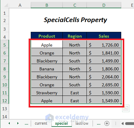
Method 3 – SpecialCells for Selecting Dynamic Range Excluding Headers
Steps:
- Follow the Steps of Method 1.
- Enter the following code:
Sub dynrange3()
Dim sht As Worksheet
Dim Lr As Long
Dim Lc As Long
Dim FirstCell As Range
Set sht = Worksheets("special")
Set FirstCell = Range("B5")
Lr = FirstCell.SpecialCells(xlCellTypeLastCell).Row
Lc = FirstCell.SpecialCells(xlCellTypeLastCell).Column
sht.Range(FirstCell, sht.Cells(Lr, Lc)).Select
End Sub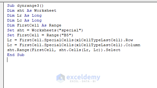
Note:
- Here, at first, we declared sht, FirstCell, Lr, and Lc as Worksheet, Range, and Long respectively.
- “special” is the worksheet name.
- “B5” is set as FirstCell because it is the starting cell of our data range.
- Lr and Lc will return the last row and column used in the worksheet.
- Finally, Range(FirstCell, sht.Cells(Lr, Lc) will give the range of the data table.
- Press F5.
- Select the whole data range, excluding headers.
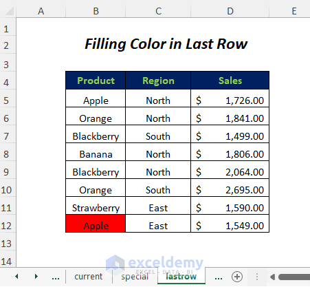
Method 4 – Change the Color for the Last Used Row with Excel VBA
Steps:
- Follow the Steps of Method 1.
- Enter the following code:
Sub dynrange4()
Dim Lr As Integer
Dim sht As Worksheet
Set sht = Worksheets("lastrow")
Lr = sht.Range("B" & Rows.Count).End(xlUp).Row
Range("B" & Lr).Interior.Color = vbRed
End Sub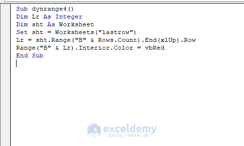
Note:
- Here, at first, we declared sht, Lr as Worksheet and Integer.
- “lastrow” is the worksheet name.
- Again, “B” means Column B because we have started our data range from this column.
- Range(“B” & Rows.Count) will select the last row number in this column and then End(xlUp) will go to the last row used in this worksheet, so it will give us the number of the row that we need in our range.
- Then, the interior color will be changed in Range(“B” & Lr), which means the last row used is in column B.
- Press F5.
- Change the color of the first cell in the last row of this data range.
Read More: How to Use Dynamic Range for Last Row with VBA in Excel
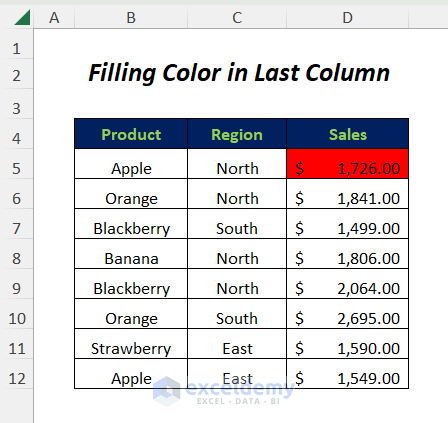
Method 5 – Edit the Color of the Last Used Column
Steps:
- Follow the Steps of Method 1.
- Enter the following code:
Sub dynrange5()
Dim Lc As Integer
Dim sht As Worksheet
Dim FirstCell As Range
Set FirstCell = Range("B5")
Set sht = Worksheets("lastcolumn")
Lc = FirstCell.SpecialCells(xlCellTypeLastCell).Column
Cells(5, Lc).Interior.Color = vbRed
End Sub
Note:
- Here, at first, we declared sht, FirstCell, and Lc as Worksheet, Range, and Long respectively.
- “lastcolumn” is the worksheet name.
- “B5” is set as FirstCell because it is the starting cell of our data range.
- Lc will return the last used column in the worksheet.
- Cells(5, Lc) will select the first cell in the last column, and here, 5 and Lc are the row and column numbers, respectively.
- Press F5.
- Change the color of the first cell in the last column of this data range.
Read More: Dynamic Range for Multiple Columns with Excel OFFSET
Method 6 – Change the Color for the Last Used Row and Column
Steps:
- Follow the Steps of Method 1.
- Enter the following code:
Sub dynrange6()
Dim Lc As Integer
Dim Lr As Integer
Dim sht As Worksheet
Set sht = Worksheets("rowandcolumn")
Lr = sht.Range("B" & Rows.Count).End(xlUp).Row
Lc = Range("XFD" & Lr).End(xlToLeft).Column
Range(Cells(5, Lc), Cells(Lr, Lc)).Interior.Color = vbGreen
End Sub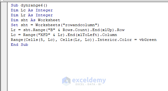
Note:
- Here, at first, we declared sht, Lr, and Lc as Worksheet, Integer.
- “rowandcolumn” is the worksheet name.
- Here, “B” means Column B because we have started our data range from this column.
- Range(“B” & Rows.Count) will select the last row number in this column and then End(xlUp) will go to the last row used in this worksheet, so it will give us the number of rows that we need in our range.
- “XFD” is the last column name and Range(“XFD” & Lr) will select the last column to the last row.
- Then End(xlToLeft) will go to the last column used in this worksheet, giving us the number of columns that we need in our range.
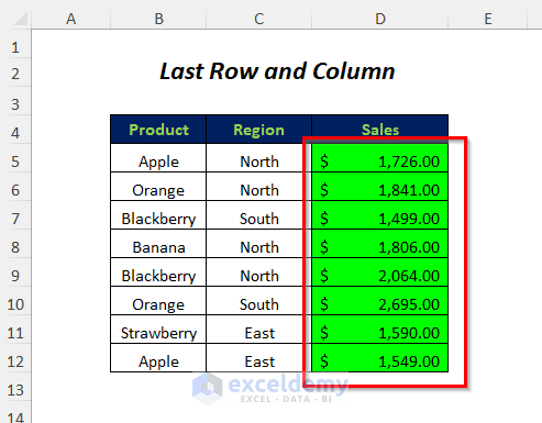
- Range(Cells(5, Lc), Cells(Lr, Lc)) is the range between the first cell of the last column and the last cell of the last column in this data range.
- Press F5.
- Change the color of all the cells in the last column of this data range.
Read More: How to Create a Range of Numbers in Excel
Method 7 – Dynamic Range VBA for Static Column
Steps:
- Follow the Steps of Method 1.
- Enter the following code:
Sub dynrange7()
Dim sht As Worksheet
Dim LR As Long
Dim FirstCell As Range
Set sht = Worksheets("staticcolumn")
Set FirstCell = Range("B5")
LR = sht.Cells.Find("*", SearchOrder:=xlByRows, _
SearchDirection:=xlPrevious).Row
sht.Range("B5:D" & LR).Select
End Sub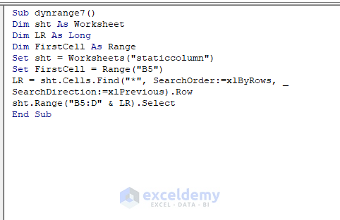
Note:
- Here, at first, we declared sht, LR, and FirstCell as Worksheet, Long, and Range respectively.
- “staticcolumn” is the worksheet name and “B5” is set as FirstCell because it is the starting cell of our data range. Find will search for any character in the data range, and so where the last character will be found, it will be the last row.
- SearchOrder:=xlByRows searches for the value row by row and returns the position of the string that comes first in the row-wise serial.
- Similarly, SearchDirection:=xlPrevious will start the search in the bottom right-hand corner of the data range and search upwards, so it will give the position of the string that comes last.
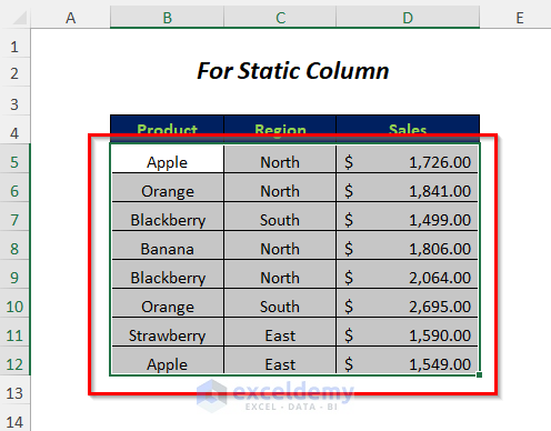
- Range(“B5:D” & LR) is the range of the data table for Column B to D and starts from row 5 to the last used row.
- Press F5.
- Select the cells of this data range.
Method 8 – Copy Data for Dynamic Range with VBA
Steps:
- Follow the Steps of Method 1.
- Enter the following code:
Sub dynrange8()
Dim sht As Worksheet
Dim LR As Long
Dim FirstCell As Range
Set sht = Worksheets("copy")
Set FirstCell = Range("B5")
LR = sht.Cells.Find("*", SearchOrder:=xlByRows, _
SearchDirection:=xlPrevious).Row
sht.Range("B5:D" & LR).Copy
End Sub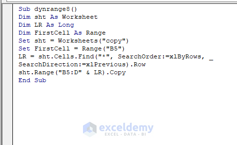
Note:
- We declared sht, LR, and FirstCell as Worksheet, Long, and Range, respectively.
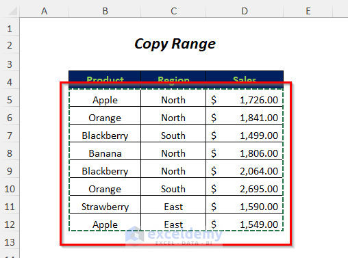
- “copy” is the worksheet name, and Range(“B5:D” & LR) is the range of the data table for Column B to D, starting from row 5 and ending with the last used row. Finally, this range will be copied.
- Press F5.
- Copy the data range.
Read More: Data Validation Drop Down List with Excel Table Dynamic Range
Method 9 – Enter Data for Dynamic Cell Range
Steps:
- Follow the Steps of Method 1.
- Enter the following code:
Sub dynrange9()
Dim Lr As Long
Dim sht As Worksheet
Set sht = Worksheets("enter")
Lr = sht.Cells.Find("*", SearchOrder:=xlByRows, _
SearchDirection:=xlPrevious).Row
Range(Cells(5, 5), Cells(Lr, 5)).Value = "January"
End Sub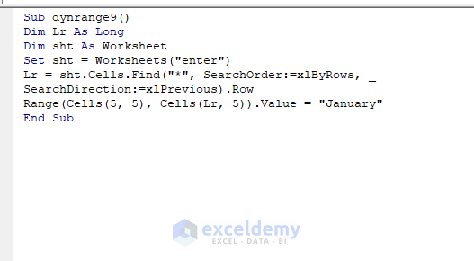
Note:
- At first, we declared sht and LR as Worksheet and Long, respectively. “enter” is the worksheet name.
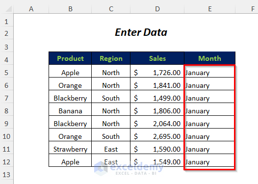
- The range (Cells(5, 5), Cells(Lr, 5)) is the data between cells E5 and E12 (it will change automatically depending on the last used row), and then the desired value will be entered in this range.
- Press F5.
- Enter the month name January in the Month column.
Read More: Excel VBA: Dynamic Range Based on Cell Value
Method 10 – Get the Last Used Dynamic Cell’s Address
Steps:
- Follow the Steps of Method 1.
- Enter the following code:
Sub dynrange10()
Dim Lc As Integer
Dim Lr As Integer
Dim rng As Range
Dim sht As Worksheet
Set sht = Worksheets("range")
Lr = sht.Range("B" & Rows.Count).End(xlUp).Row
Lc = Range("XFD" & Lr).End(xlToLeft).Column
Set rng = Range(Cells(5, 2), Cells(Lr, Lc))
MsgBox "The range is " & rng.Address
End Sub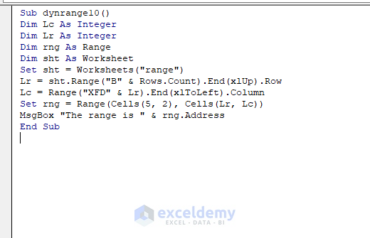
Note:
- First, we declared sht, Lr, Lc, and rng as Worksheet, Integer, and Range, respectively. “range” is the worksheet name.
- Range(Cells(5, 2), Cells(Lr, Lc)) is the range between the starting cell B5 and the last cell having the last used row and column number in the range. Then, it will be set as rng, and finally, it will give the range address.
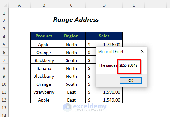
- We used MsgBox to present the output through a message box.
- Press F5.
- Get the range address as $B$5:$D$12 for the following data range.
Read More: Dynamic Named Range Based on Cell Value in Excel
Method 11 – Dynamic Range for Tables
Steps:
- Go to Insert Tab>>Table Option.
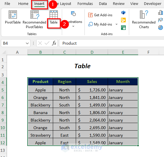
- The Create Table Dialog Box will open up.
- Select the data range.
- Click on the Option named My table has headers.
- Press OK.
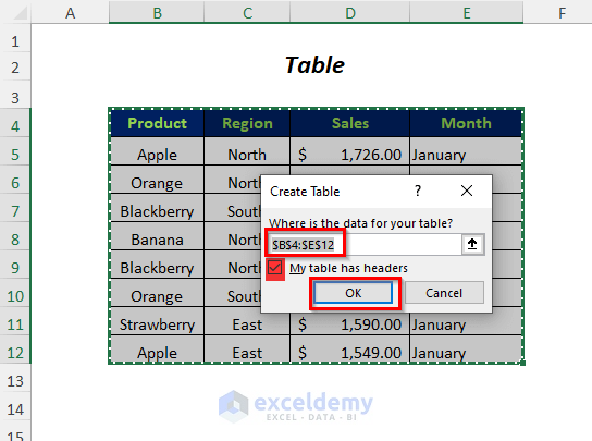
- You will get the following data table.

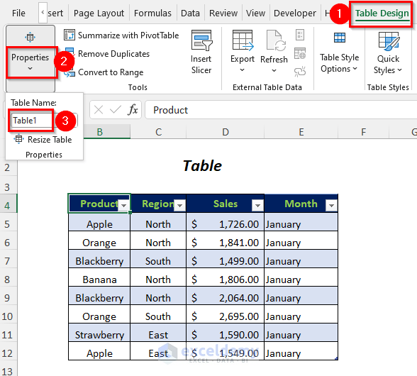
- Go to Table Design Tab>>Properties Option.
- Write any name in the Table Name Box (Here, I have used Table1).
- Follow the Steps of Method 1.
- Enter the following code:
Sub dynrange11()
ActiveWorkbook.Worksheets("Table").ListObjects("Table1").ListColumns("Month").Delete
End Sub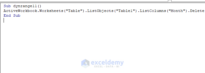
Note:
Here, Table is the worksheet name, Table1 is the table name and Month is the column name that you want to delete.
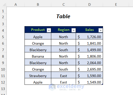
- Press F5.
- Delete the column Month.
Download the Workbook
You can download the workbook used for the demonstration from the download link below.
Related Articles
- OFFSET Function to Create & Use Dynamic Range in Excel
- How to Create Dynamic Range Using Excel INDEX Function
- Create Dynamic Sum Range Based on Cell Value in Excel
- How to Autofill Dynamic Range Using VBA in Excel

