How to Write Code in the Visual Basic Editor
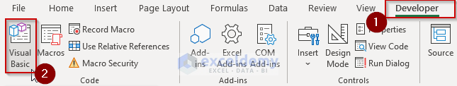
- Go to the Developer tab from the Excel Ribbon.
- Click the Visual Basic option.
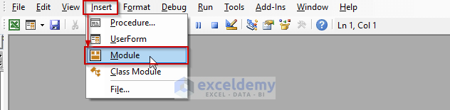
- In the Visual Basic for Applications window, click the Insert dropdown to select the Module option.
- Write or insert your code in the Module and use F5 to run it.
Example 1 – Select a Dynamic Range Based on the Value of Another Cell Using VBA in Excel
We have a list that contains city names in cells A1:A7 with their country names in the next column (cells B1:B7). We want to configure a code that will select multiple rows from these two columns. The number of rows to be selected should not be hardcoded but dynamic based on a cell value.
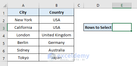
- In cell E3, we’re going to put the number of rows (in this example, 3) to select.
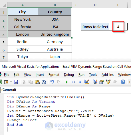
- Copy and paste the following code into the visual code editor.
Sub DynamicRangeBasedOnCellValue()
Dim DValue As Variant
Dim DRange As Range
DValue = ActiveSheet.Range("E3").Value
Set DRange = ActiveSheet.Range("A1:B" & DValue)
DRange.Select
End Sub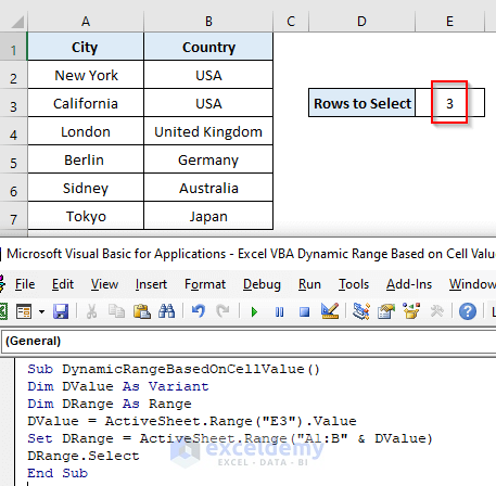
- Press F5 to run the code.
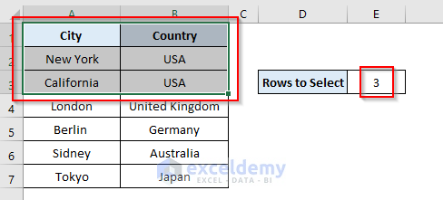
- We’ve successfully selected the first three rows of the dataset. If we put 4 in cell E3 and run the code again, we’ll get four rows.
Read More: How to Use Dynamic Range for Last Row with VBA in Excel
Example 2 – Define a Dynamic Range Based on Cell Values Using VBA in Excel
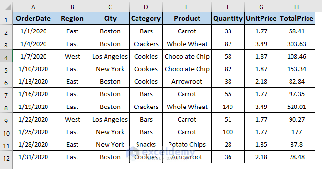
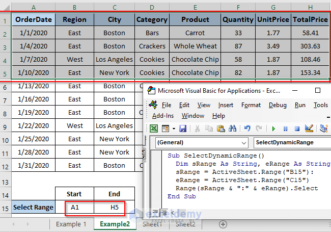
In this example, we’ll show how to define and then select a dynamic range based on two cell values i.e., one cell value to define the starting and another to the end of the dynamic range. To illustrate this, let’s count in the following dataset ranging from A1:H12. We’ve specified two cells in the worksheet, B15 and C15, from where we’re going to take the starting and ending range data of our dynamic range in our VBA code.
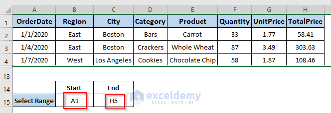
- We need to define two cells that hold the starting and end of the dynamic range. We defined cells B15 and C15 to hold the starting and end of the range i.e., A1 to H5 in this example.
- Copy and paste the following code into the visual code editor.
Sub SelectDynamicRange()
  Dim sRange As String, eRange As String
  sRange = ActiveSheet.Range("B15"):
  eRange = ActiveSheet.Range("C15")
  Range(sRange & ":" & eRange).Select
End Sub
In this code, we declared two different variables named sRange and eRange to hold the starting and end cell reference of the dynamic range in cells B15 and C15, respectively.
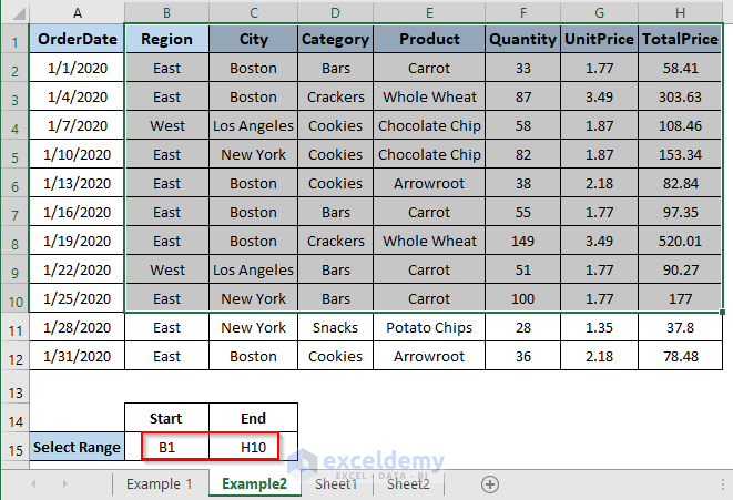
- Press F5 to run the code. We’ve successfully selected the range of Rangel A1:H5.
If we change the values of cells B15 and C15 to some other value, the selected range will change accordingly.
Example 3 – Copy and Paste a Dynamic Range Based on Cell Value with Excel VBA
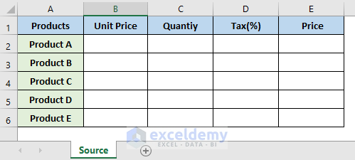
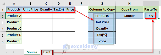
We have a demo sales info template that one shop manager has to create every day to store sales information. We’re going to copy and paste the template to a new worksheet based on a cell value that holds the worksheet name. We’ll be able to decide what portion of the template should be copied and then pasted to our desired worksheet. Here is the template in the below screenshot which is in the “Source” worksheet.
To facilitate the user to choose what columns to copy in the new worksheet, we inserted the column names in cells G2:G6. In cell H2, we put the source worksheet name, and form where we’re going to copy the template to a new worksheet. We need to put the new worksheet name in cell I2.
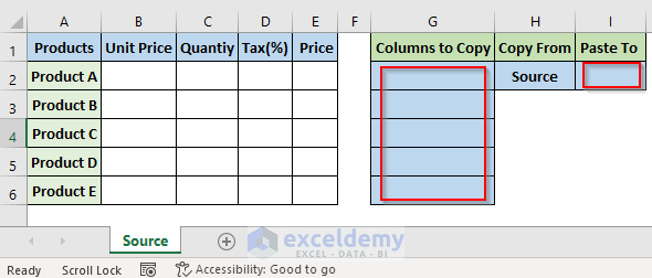
- We’ve created a new worksheet for Day 1 of a month named “Day1”.
- In cell I2, we put the new worksheet name.
- In cells G2:G6, we put the column names to copy in the worksheet named Day1.
- Copy and paste the following code in the visual code editor.
Sub CopyPasteDynamicRange()
    Dim CSheet As Worksheet, PSheet As Worksheet
    Dim CRange As Range, PRange As Range
    Dim CLastRow As Long, CLastCol As Long, PLastCol
    Dim ColArray As Variant
    Dim ColName As Variant
    Dim ColNo As Long
    Dim a, b As String
    a = ActiveSheet.Range("H2").Value
    b = ActiveSheet.Range("I2").Value
    Set CSheet = Sheets(a)
    Set PSheet = Sheets(b)
    CLastRow = CSheet.Range("A" & Rows.Count).End(xlUp).Row          ' last row
    CLastCol = CSheet.Cells(1, Columns.Count).End(xlToLeft).Column   ' last column
    With CSheet
        Set CRange = .Range(.Cells(1, "A"), .Cells(CLastRow, CLastCol))
    End With
    PLastCol = PSheet.Cells(1, Columns.Count).End(xlToLeft).Column   ' last column
    ColArray = Range("G2:G6").Value ' column headers
    For Each ColName In ColArray
        ColNo = Application.Match(ColName, CRange.Rows(1), 0)
        PLastCol = PLastCol + 1
        CRange.Columns(ColNo).Copy Destination:=PSheet.Cells(1, PLastCol)
    Next ColName
End Sub- Press F5 to run the code.
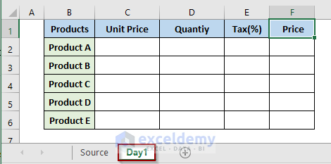
- Navigate to the worksheet named “Day1”. The output is here below.
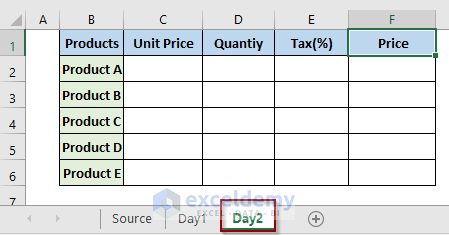
- We can make another worksheet for Day2 and run the code again after changing the I2 cell value to Day2.
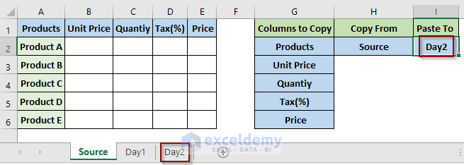
The output is:
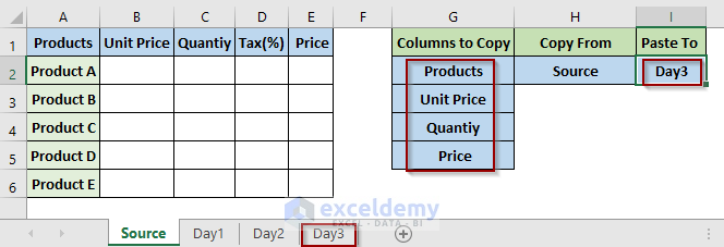
We need to copy the template without the Tax(%) column in the Day3 worksheet. We need to set up the values like this.
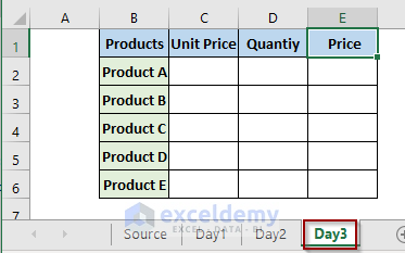
In the output, in the Day3 worksheet, we have the template but without the Tax column.
Read More: Excel VBA: Copy Dynamic Range to Another Workbook
Download the Practice Workbook
Get FREE Advanced Excel Exercises with Solutions!
