How to Use Dynamic Range for Last Row with VBA in Excel (3 Methods)

Why Do You Need a Dynamic Range

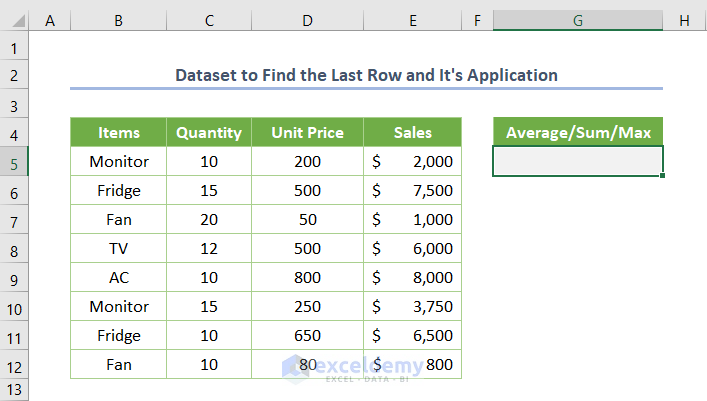
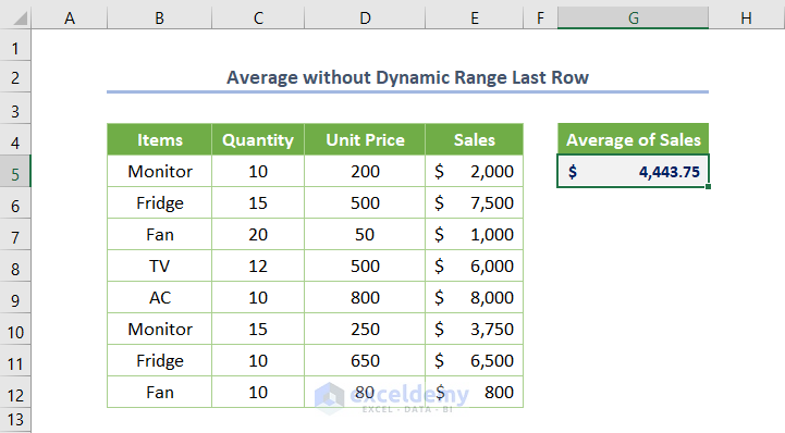
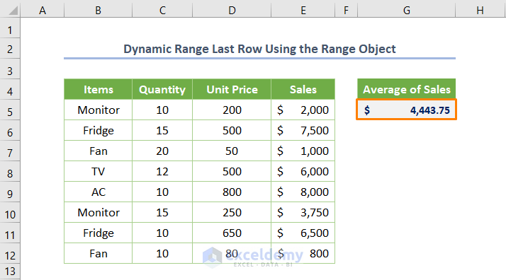
We have a simple dataset with Quantity, Unit Price, and Sales of some Items. We want to find the average, sum, maximum value, or a similar value via VBA.

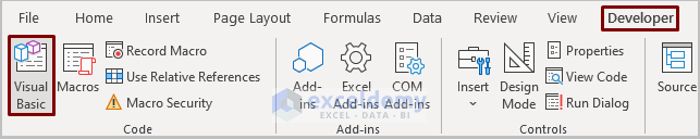
Open the VBA window by clicking Developer and selecting Visual Basic.

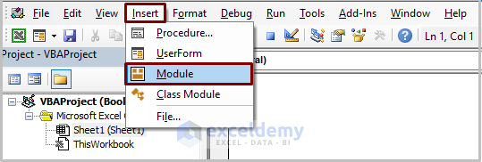
Go to Insert and choose Module.

Copy the following code into the newly created module.

Sub Average_without_DynamicRangeLastRow()
Range("G5").Value = Application.WorksheetFunction.Average(Range("E5:E12"))
End Sub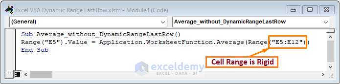

We used the Range.Value property to define the output cell. We applied WorksheetFunction.Average for computing the average of the Sales.

If you run the code (the keyboard shortcut is F5 or Fn + F5), you’ll see the following output.

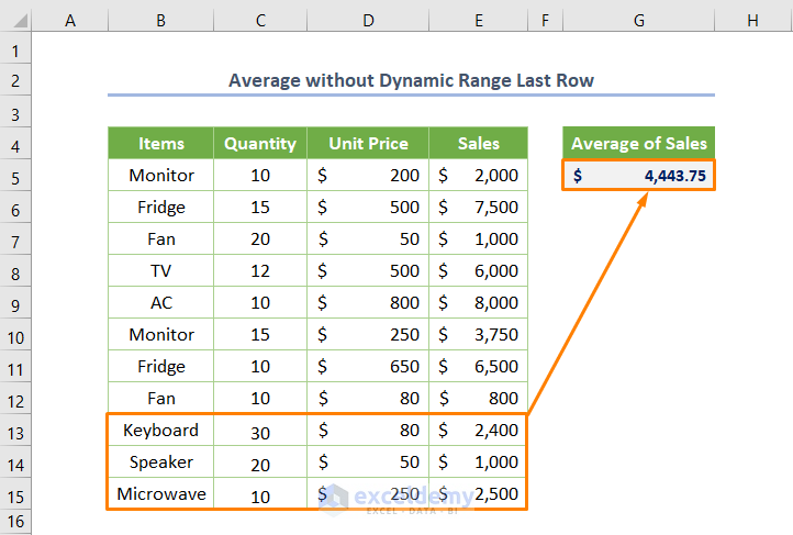
Let’s add a new entry e.g. B13:E15 cell range. However, the current code doesn’t cover it and would need to be readjusted manually. That’s why putting a dynamic range to determine the last row is valuable for larger datasets.

Excel VBA Dynamic Range for Last Row: 3 Methods to Use

Method 1 – Using the Range Object

Step 1 – Finding the Last Row

To get the number of the last row in the case of your dataset, use the following code.

Sub Dynamic_Last_Row_Method1()

Dim LRow As Long

LRow = Range("E:E").SpecialCells(xlCellTypeLastCell).Row

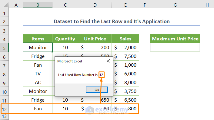
MsgBox "Last Used Row Number is: " & LRow

End Sub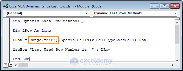

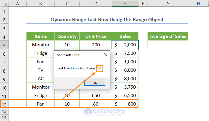
In the above code, we declared the LRow (short form of the last row) as a Long data type first. We defined the LRow with the Range (“E:E”) and SpecialCells method which would return the last cell. We utilized the Row property to get the row number. A MsgBox is added to display the last row number.

If you run the code, you’ll get the output 12.

Note: I used column E but you may insert any other column based on your requirement.

Step 2 – Computing Average

Use the following code to compute the average of the Sales.

Sub Average_Method1()

Dim LRow As Long

LRow = Range("E:E").SpecialCells(xlCellTypeLastCell).Row

Range("G5").Value = Application.WorksheetFunction.Average(Range("E5:E" & LRow))

End Sub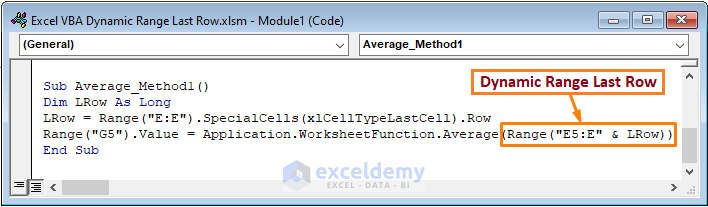

In the above code, I declared the LRow and defined its value. More importantly, I added Column E (which holds the value of the Sales) along with the LRow to get the average of the Sales field in the G5 cell of the sheet.

Note: Remember this same code will work for calculating the average no matter if you add new data or remove any data from the existing dataset.

After running the code, you’ll get the average of the Sales is $4443.75.

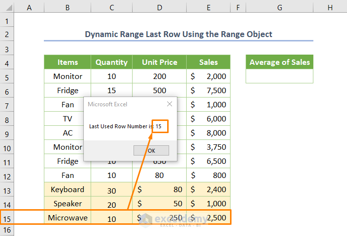
Step 3 – Dealing with Newly Added Data

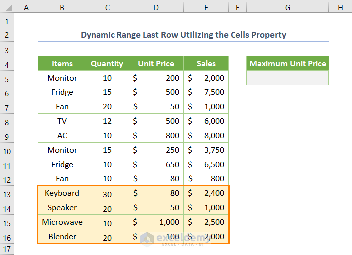
We added new entries e.g. B13:E15 cells.
We ran the code from Step 1 and got the result 15.

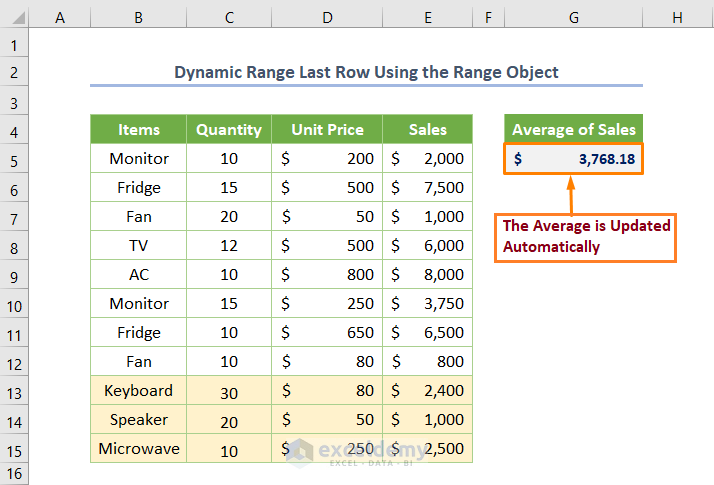
Running the code from Step 2 gives the updated result.

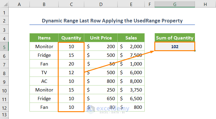
Method 2 – Applying the UsedRange Property

Step 1 – Computing Sum in the Usual Way

To compute the sum for a cell range, use the following code.

Sub Sum_Quantity_without_DynamicRangeLastRow()

Range("G5").Value = WorksheetFunction.Sum(Range("C5:C12"))

End Sub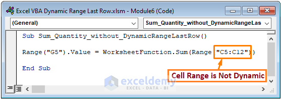

In the above code, we used the WorksheetFunction.Sum method with defining the C5:C12 cell range. However, the cell range is not dynamic. That means you have to change the cell range if you add new data to the dataset.

Step 2 – Finding the Last Row

This code fetches the last row in the range.

Sub Dynamic_LastRow_Method2()

Dim LRow As Long

LRow = ActiveSheet.UsedRange.Rows(ActiveSheet.UsedRange.Rows.Count).Row

MsgBox "Last Used Row Number is: " & LRow

End Sub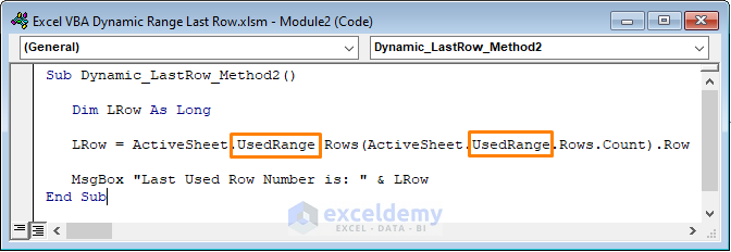

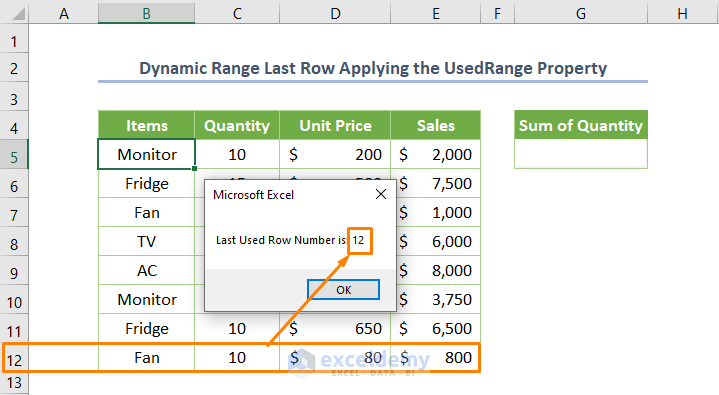
In the above code, we defined the LRow with the UsedRange which displays the last used range on a certain worksheet. Then Rows.Count counts the total number of rows in the active worksheet.

After running the code, the output will be 12.

Step 3 – Dealing with Newly Added Data and Computing the Sum

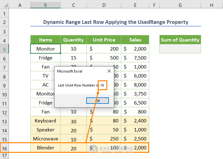
Let’s say, you want to add 4 new rows (B13:E16 cell range). After adding the new rows, if you run the same code mentioned in the previous step, you’ll get the changed row number is 16.

To get a sum of cells starting from E5 and ending with the last filled row in the column, copy the following code.

Sub Sum_Method2()

Dim LRow As Long

LRow = ActiveSheet.UsedRange.Rows(ActiveSheet.UsedRange.Rows.Count).Row

Range("G5").Value = Application.WorksheetFunction.Sum(Range("C5:C" & LRow))

End Sub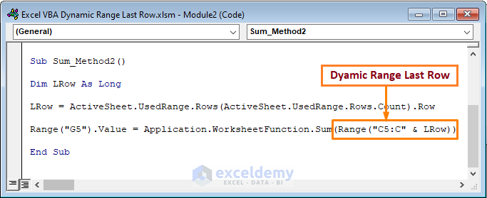

We specified the Quantity field (column C) with the dynamic LRow.

You’ll get the sum of the Quantity is 182 if you run the code.

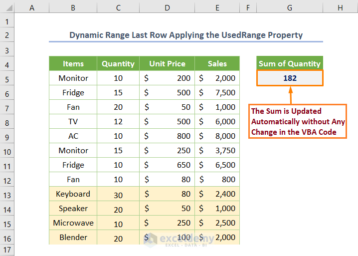
Needless to say the code will work dynamically and you don’t need to make any changes to the code.

Method 3 – Utilizing the Cells Property

Step 1 – Finding the Last Row

Copy the following code to find the last row.

Sub Dynamic_LastRow_Method3()

Dim LRow As Long

LRow = Cells(Rows.Count, 4).End(xlUp).Row

MsgBox "Last Used Row Number is: " & LRow

End Sub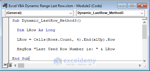

In the above code, we assigned Rows.Count and the value of 4 (the column number is of column D) in the Cells property. That means it counts all the row numbers of column D. We used the End property with the xlUp snippet which finds the last used row.

Step 2 – Working with the Dynamic Range in the Last Row

Add the new data as shown in the following image.

Use the following code to get the maximum price.

Sub Max_Price_Method3()

Dim LRow As Long

LRow = Cells(Rows.Count, 4).End(xlUp).Row

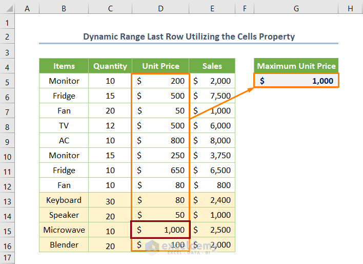
Range("G5").Value = Application.WorksheetFunction.Max(Range("D5:D" & LRow))

End Sub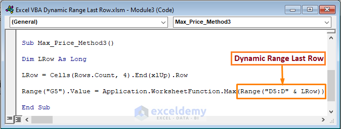

We utilized the WorksheetFunction.Max method to return the maximum value in column D.