Dynamic Range for Multiple Columns with Excel OFFSET

A dynamic range expands automatically when you update the raw data in the range. In this article, we’ll discuss the ways to apply the OFFSET function in a dynamic range and dynamic named range for multiple columns. We’ll also show how to use the INDEX and MATCH functions as an effective alternative.

The OFFSET Function

The OFFSET function returns a cell or cell range where the starting point, number of rows and columns, height, and width are provided.

The syntax of the function is

The arguments are-
reference – The starting point, given as a cell reference or range.
rows – The number of rows to offset below the starting reference.
cols – The number of columns to offset to the right of the starting reference.
height – The height in rows (optional).
width – The width in columns (optional).

Create Dynamic Range for Multiple Columns Using Excel OFFSET: 2 Ways

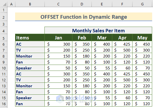
In our sample dataset we have some electronic Items and their monthly sales from January to May.

Method 1 – Dynamic Range Using OFFSET and COUNT Functions

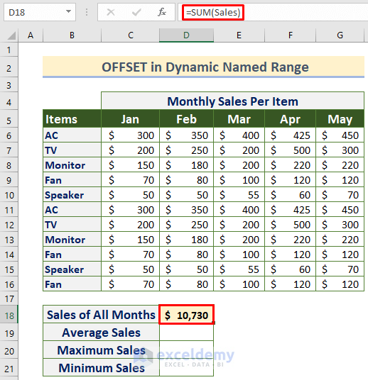
Let’s utilize the OFFSET function to calculate the total sales of all items in January and February

Steps:

• In cell D18, enter the following formula:

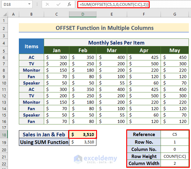
The COUNT function counts the number of cells in column C with numbers, providing the Row Height for the OFFSET function.

For reference, the parameters for the OFFSET function are provided in the highlighted box in the image above, and in cell D19 we check our result using the SUM function:

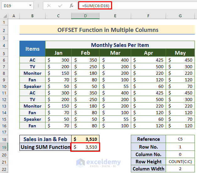
• To find the sales of all items in all months, select cell D18 and insert the following formula in the Excel formula bar:

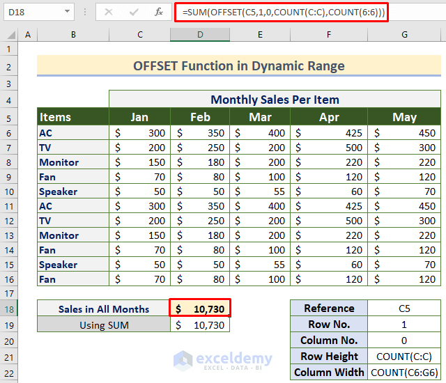
Now let’s add sales for all items in a new month to our dataset, namely June in column H. If the previous formula works on the updated data, then the OFFSET function is working efficiently.

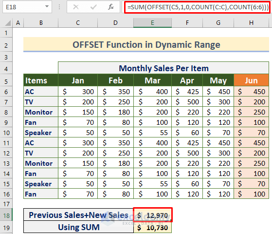
The sales data is updated automatically to include June’s sales without needing to update the OFFSET formula. But in the case of the SUM function, it remains unchanged.

This is possible because we set the values of Height and Width as the entire column C and row 6.

Read More: Create Dynamic Sum Range Based on Cell Value in Excel

Method 2 – Dynamic Named Range Using Excel OFFSET and COUNT Functions

A dynamic named range is created by defining the name of any cell range. This name can be then be used in our the formulas in place of the cell references it represents.

Steps:

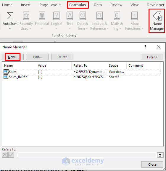
• Open the Name Manager dialog box by clicking Formulas >> Named Manager.
• Click New to set a new range name.

• Type a name in the Name option, and the following formula in the Refers to section:

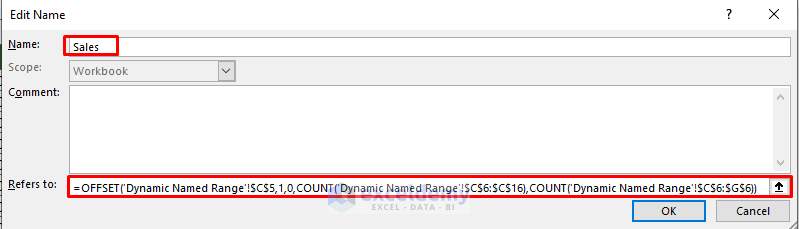
A named range for the range reference of the OFFSET function is created.

Alternatively, you can insert the formula by clicking the lower right portion (Up Directional Key) of the above dialog box.

Now the formula can be specified without any confusion about ranges or references.

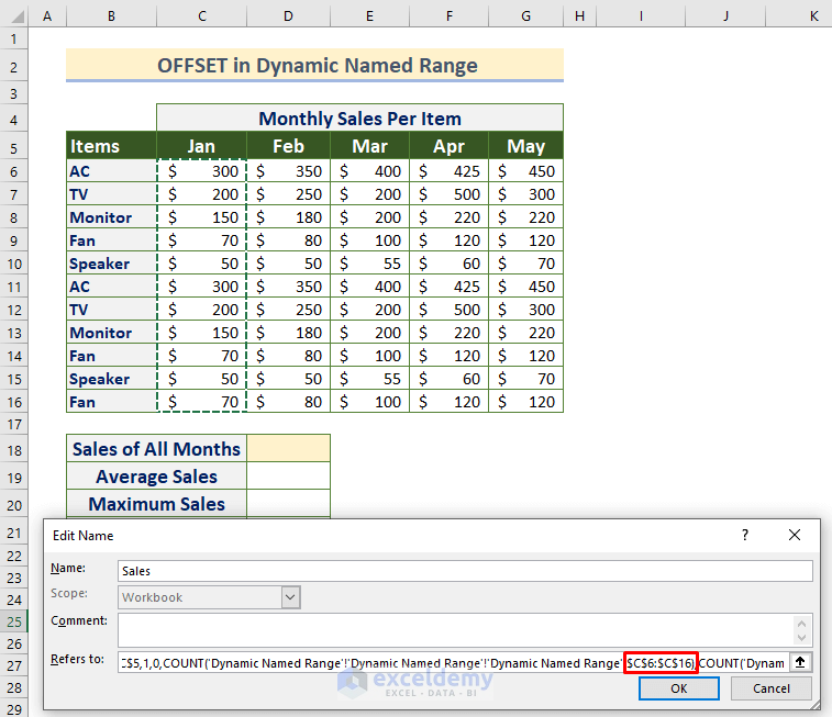
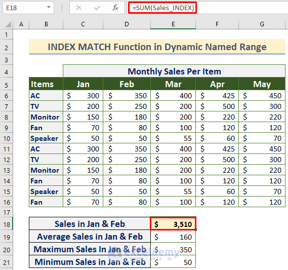
• Select a cell to store the Sales of the entire month and enter the following formula in it:

• Press ENTER to return the total Sales amount in that range.

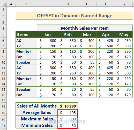
Similarly, we can find the average, maximum, and minimum value of the sales for all items using the AVERAGE, MAX, and MIN functions respectively as shown in the following illustration.

Read More: OFFSET Function to Create & Use Dynamic Range in Excel

An Effective Alternative: Using INDEX and MATCH for Dynamic Range

We can also utilize the INDEX MATCH function, a popular combination of two functions, to make calculations on a specified dynamic range. In the case of a larger dataset, the OFFSET function performs slowly, so this method will be more effective.

Steps:

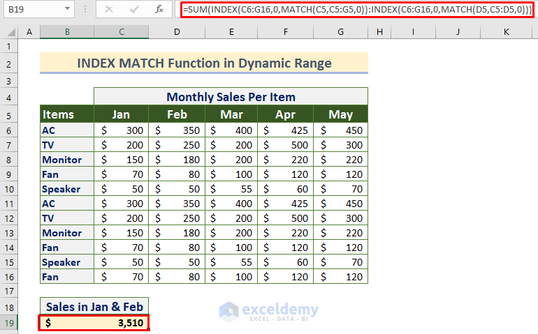
• Calculate the sum of Sales in January and February for all items with the following formula:

Here, C6:G16 is the cell range for the sales of all items, C5 is for the month i.e. January, C5:G5 is the cell range for five months, and D5 is for the month i.e. February.

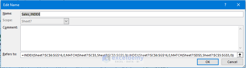
• Insert the following formula in the same way as we inserted the OFFSET function above:

The following dialog box appears.

• Do the analysis as required e.g. sum, average etc.

Read More: How to Create Dynamic Range Using Excel INDEX Function

Things to Keep in Mind

• Be careful while inserting the formula in the Named Manager. If there is any parenthesis or referring problem, you will get a #VALUE error in doing the analysis.
• If the cell value or range is not fixed by using $ (dollar sign) and the formula takes the cell range out of your dataset, you will receive a #REF error.

Download Practice Workbook

Further Readings

• Data Validation Drop Down List with Excel Table Dynamic Range
• How to Create a Range of Numbers in Excel
• Dynamic Named Range Based on Cell Value in Excel

<< Go Back to Dynamic Range | Named Range | Excel Formulas | Learn Excel