How to Find Intersection of Two Trend Lines in Excel (3 Methods)

An intercept of two trendlines represents the solution for these equations and you may need to find that point using Excel. So, if you are looking for how to find that common point of two trend lines in Excel then you have come to the right place. Today, I will demonstrate how to find the intersection of two trend lines in Excel.
Furthermore, for conducting the session, I will use the Microsoft 365 version.

What Is Trendline?

A Trendline is a statistical pattern used for knowing the trend or what the dataset is denoting. It is made by putting a straight line between the high and low points of the dataset. Actually, you can use a Trendline Equation to determine a curve that provides the most accurate fit to a set of data points. Furthermore, with the help of Excel, you can find different types of curves for Trendline according to your preference.

How to Find Intersection of Two Trend Lines in Excel: 3 Methods

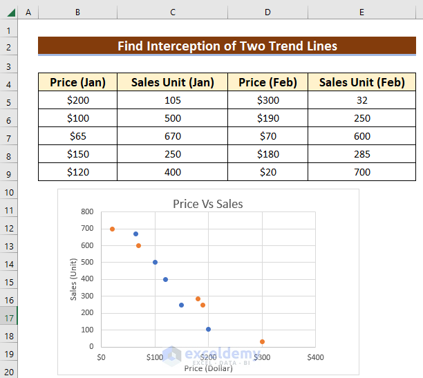
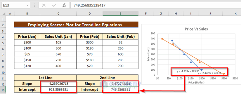
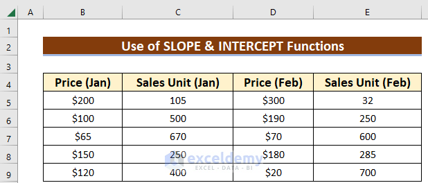
Here, I will describe 3 suitable methods to find out the interception of two trendlines in Excel. In addition, for your better understanding, I will use a sample dataset, which contains four columns along with the scatter plot. Basically, these columns represent some collected data of a company about the price and quantity of sales for the month of January and February. The dataset is given below.

1. Use Trend Line Equations to Get an Intersection Point in Excel

You can use the Trendline equations from the Chart Elements feature to get the slope and intercept of those two trendlines in Excel. Furthermore, using these, you can find the coordinates of the intersection point. Now, follow the steps given below.

Steps:

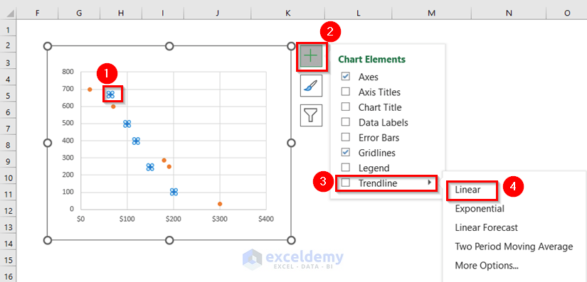
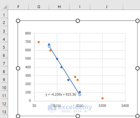
• Firstly, click on the scatter points of the 1st curve.
• Secondly, from the Plus (Chart Elements) icon >> go to Trendline >> choose Linear.

Consequently, you will see the trendline for the 1st curve.

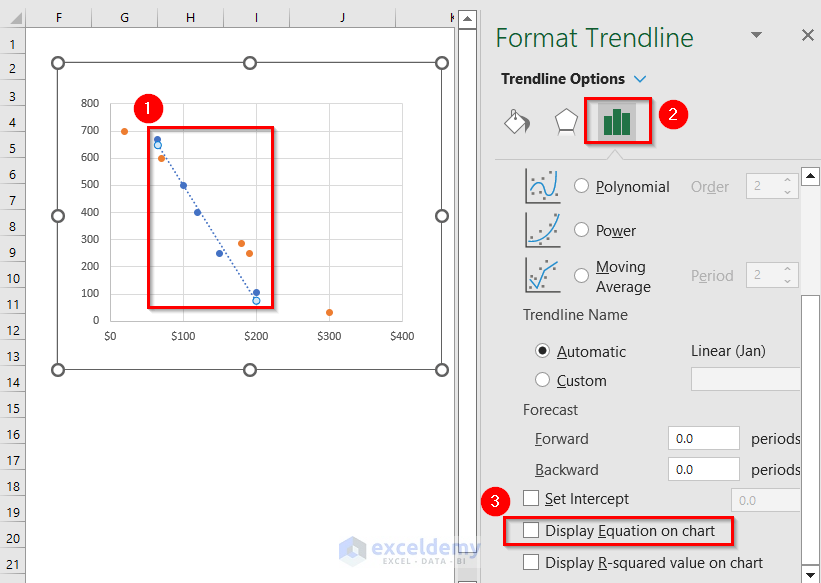
• Then, double-click on that line.

As a result, a new window named Format Trendline will appear on the rightmost side of the Excel sheet.

• Now, from Trendline Options >> check Display Equation on chart.

• Furthermore, from the Fill & Line menu >> you can change the Dash type to Solid line.

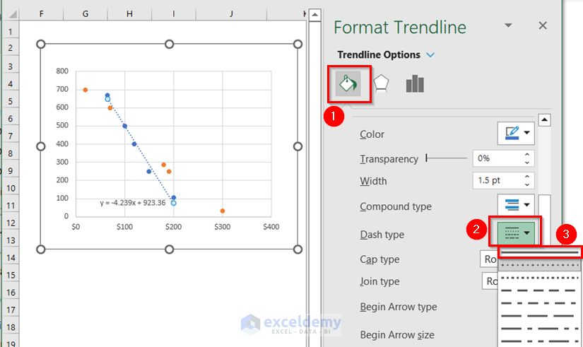
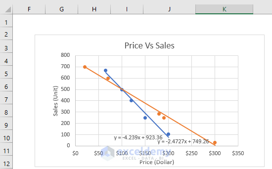
• Lastly, you will get the equation of the 1st Trendline.

Basically, the equation format is Y=mX+c. Where m is the slope, and c is the intercept.

• Similarly, find the equation for the 2nd Trendline.

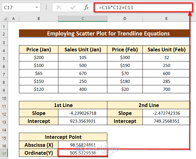
• Then, manually insert the values of slope and intercept for both lines using the equations. Here, you have to insert the values along with the sign. Furthermore, slopes are the coefficient of X and intercepts are the constant terms of the equations.

At this time, I will find out the coordinates of that intercept point.

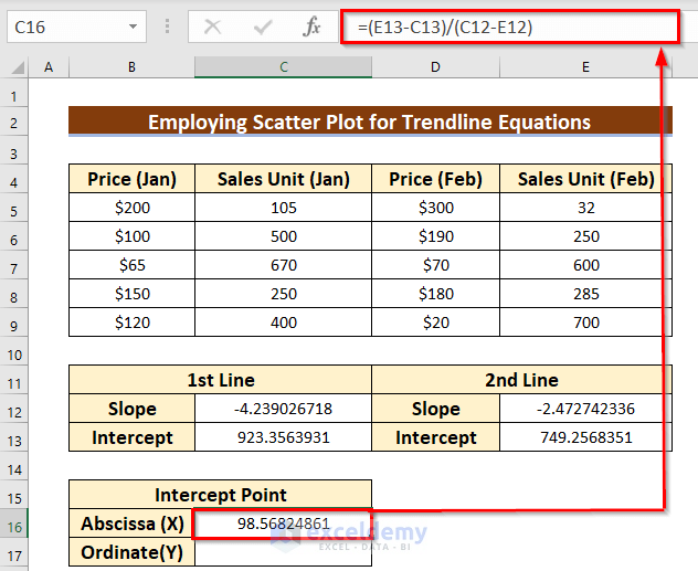
• So, in the C16 cell, use the following formula.

• Then, press ENTER, and you will get the abscissa (X) of that point.

• Then, apply the formula given below in the C17 cell.

• Lastly, press ENTER, and you will get the ordinate (Y) of that point.

Read More: How to Add Trendline Equation in Excel

2. Apply Goal Seek Feature to Calculate an Intersection Point of Two Trendlines

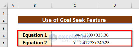
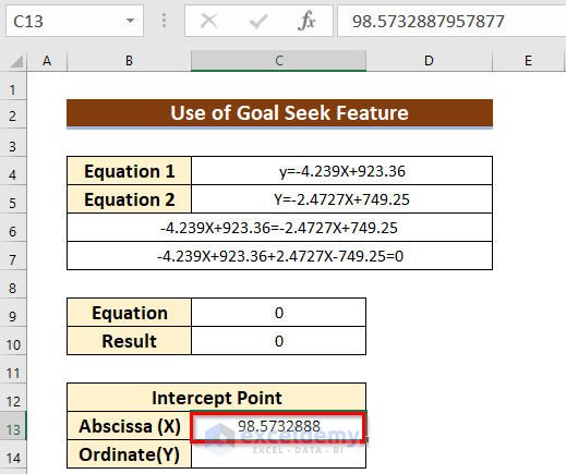
Here, you can employ the Goal Seek feature under the Data tab to find the common point or intersection of two lines in Excel. Suppose you have the following two equations. At this moment, you want to know the intersection point of them.

Now, let’s see the steps.

Steps:

• At first, equate these equations in the B6 cell using the Apostrophe (‘). Here, I have merged B6:D6 cells. Here, the Apostrophe (‘) denotes that this is a text. Otherwise, you can’t equate these equations directly using an equal sign (=) in Excel. 

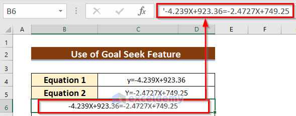
• Then, move the right-hand side to the left-hand side, using the equation law.

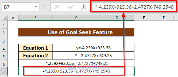
• After that, use the C13 cell reference instead of X in the above equation and keep this in the C9 cell.

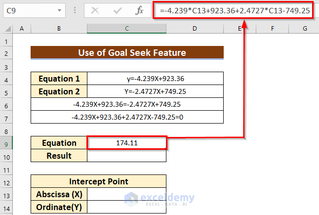
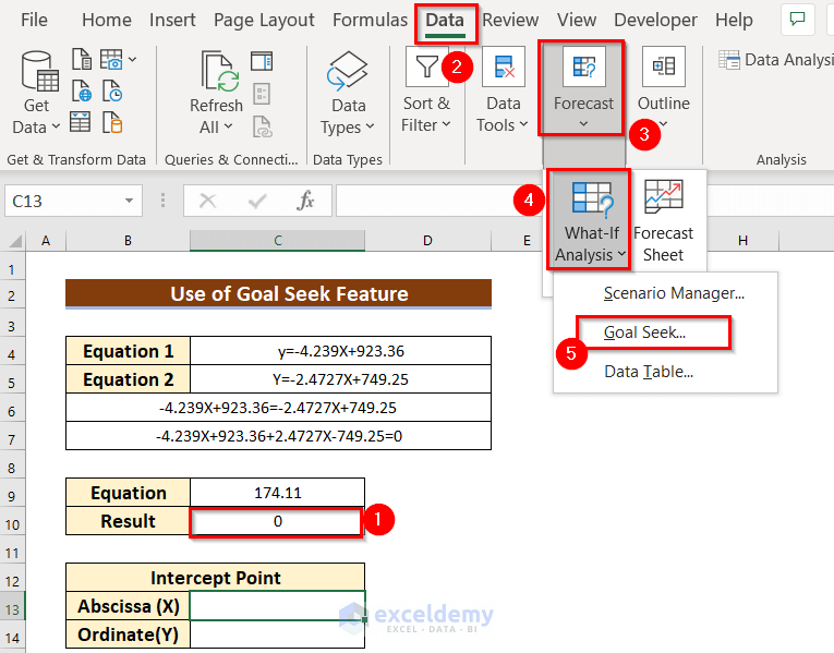
• Now, write “0” in the C10 cell as the equation must be equal to zero.
• Then, from the Data tab >> go to Forecast >> then from What-If Analysis >> choose the Goal Seek feature.

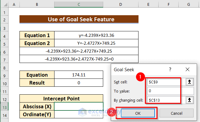
As a result, a new dialog box named Goal Seek will appear.

• Firstly, use the C9 cell reference in the Set cell box.
• Secondly, write 0 in the To value box.
• Thirdly, select the C13 cell in the By changing cell box.
• Lastly, press OK.

Subsequently, another dialog box named Goal Seek Status will pop up.

• Here, press OK.

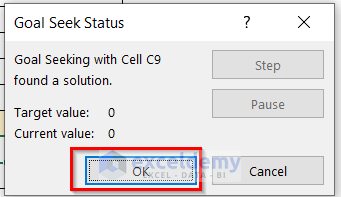
As a result, you will see the abscissa (X) of that intercept point in the C13 cell.

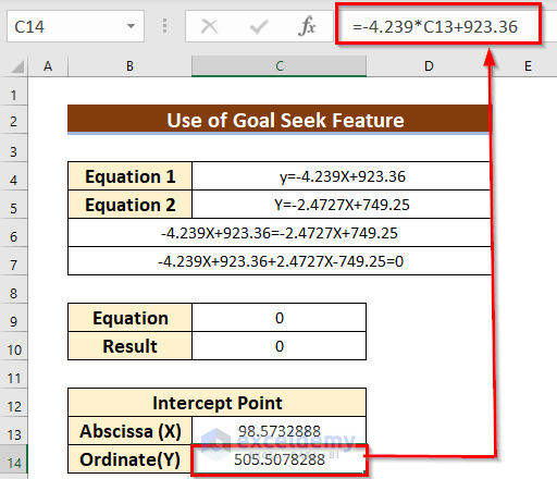
• Lastly, apply the following formula in the C17 cell.

Basically, I have used the C13 cell value (X) in the 1st equation to find the Y value.

• After pressing ENTER, you will get the ordinate (Y) of that point.

Read More: How to Get Y Equation on Excel Graph

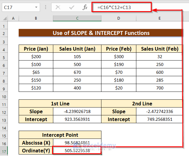
3. Combine INTERCEPT & SLOPE Functions to Find an Intersection Point of Two Trend Lines

You can use a combination of SLOPE and INTERCEPT functions to find the intersection of two trendlines in Excel. Along with this, you have to use two generic formulas to find the point of interception.
Furthermore, you can use this method when you have the points of the trend lines. So, suppose, you have the following dataset of points.

Now, let’s follow the steps.

Steps:

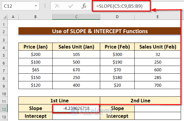
• Firstly, you must select a new cell C12 where you want to keep the slope of the 1st trend line.
• Secondly, you should use the formula given below in the C12 cell.

Here, in this formula, the SLOPE function will return the slope of the specified equation. Where C5:C9 is the y values range and B5:B9 is the x values range.

• Thirdly, press ENTER.

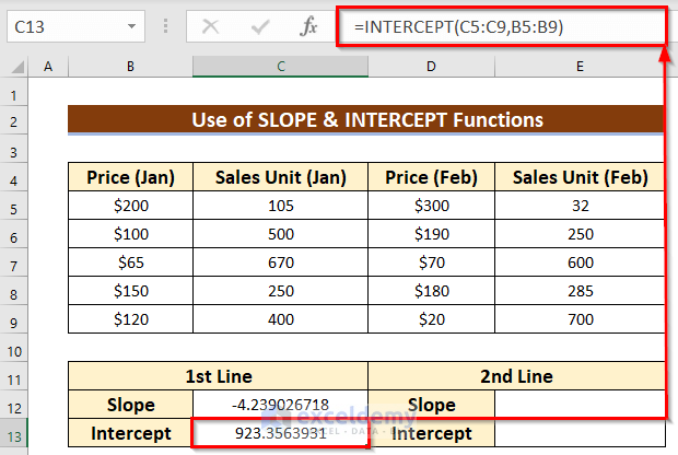
• After that, write down the corresponding formula in the C13 cell to find the intercept of the 1st trend line.

In this formula, the INTERCEPT function will give the intercept of the specified equation using regression analysis. Where C5:C9 is the y values range and B5:B9 is the x values range.

• Then, press ENTER to get the intercept of the 1st trend line.

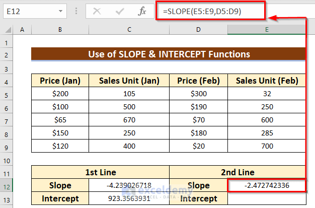
• In the same way, write down the formula given below in the E12 cell to find the slope of the 2nd trend line.

Here, in this formula, the SLOPE function will return the slope of a certain equation. Where E5:E9 is the y values range and D5:D9 is the x values range.

• Then, press ENTER to get the slope of the 2nd trend line.

• Similarly, write down the corresponding formula in the E13 cell to find the intercept of the 2nd trend line.

Basically, in this formula, the INTERCEPT function will give the intercept of the specified equation using regression analysis. Where E5:E9 is the y values range and D5:D9 is the x values range.

• Consequently, press ENTER to get the intercept of the 2nd trend line.

At this time, I will find out the coordinates of that intersection point.

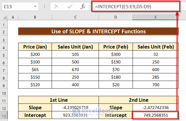
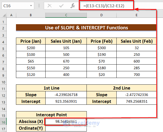
• So, in the C16 cell, use the following formula.

• Then, press ENTER, and you will get the abscissa (X) of that point.

• Then, apply the formula given below in the C17 cell.

• Finally, press ENTER, and you will get the ordinate (Y) of that point.

🗒️Things to Remember

• Here, you should use method 1 (use Trendline equation from Chart Elements) when you have the chart as a dataset.
• Furthermore, you can use method 2 (Goal Seek feature) when you have the trendline equations as given information.
• Moreover, you might use method 3 (combination of SLOPE & INTERCEPT functions) if you have the points of two trendlines as the dataset.

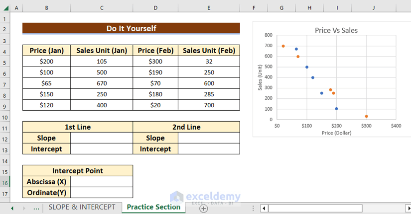
Practice Section

Now, you can practice the explained method by yourself.

Download Practice Workbook

Download this practice sheet to practice while you are reading this article.

Conclusion

I hope you found this article helpful. Here, I have explained 3 suitable methods to find the interception of two trend lines in Excel. Please, drop comments, suggestions, or queries if you have any in the comment section below.

Related Articles

• How to Find the Equation of a Line in Excel
• How to Find the Equation of a Trendline in Excel
• How to Show Equation in Excel Graph
• How to Create Equation from Data Points in Excel
• How to Use Trendline Equation in Excel
• How to Find Slope of Trendline in Excel
• How to Find Slope of Polynomial Trendline in Excel