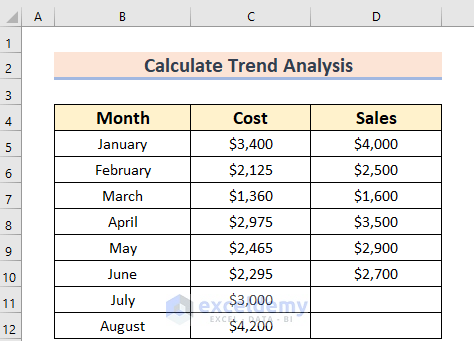
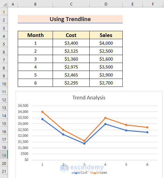
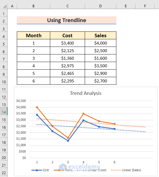
The following dataset contains three columns: Month, Cost, and Sales.
Method 1. Using the TREND Function to Calculate Trend Analysis in Excel
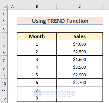
This is the sample data. There are two columns: Month and Sales.
Steps:
- Select a different cell (D5, here) to calculate the Trend analysis.
- Enter this formula.
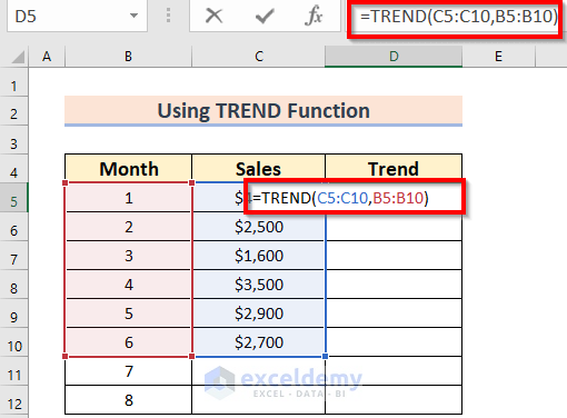
TREND will return a value in a linear way with the given points using the least square method. In this function,
-
- C5:C10 is the known dependent variable, y.
- B5:B10 is the known independent variable, x.
- Press ENTER or CTRL+SHIFT+ENTER.
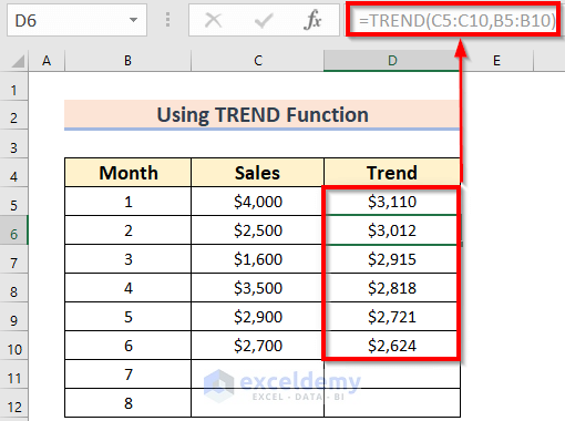
This is the output.
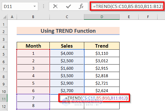
To forecast Sales for the Months of July and August:
- Select a different cell (D11, here) to calculate the Trend analysis.
- Enter this formula.
Here:
-
- C5:C10 is the known dependent variable, y.
- B5:B10 is the known independent variable, x.
- B11:B12 is the new independent variable, x.
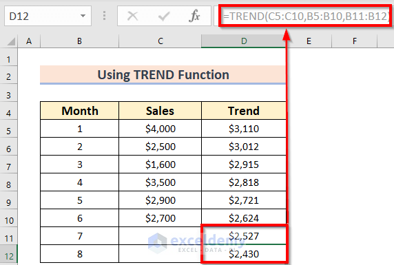
- Press ENTER.
This is the output.
Read More: How to Add Trendline in Excel Online
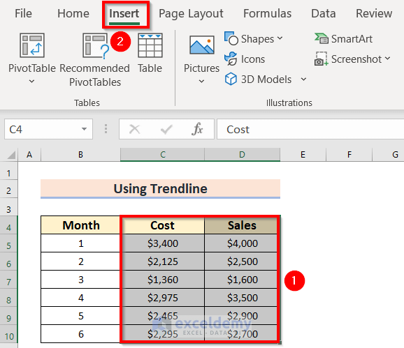
Method 2 – Using the Excel Charts Group
Steps:
- Select the data. Here, C4:D10.
- Go to the Insert tab.
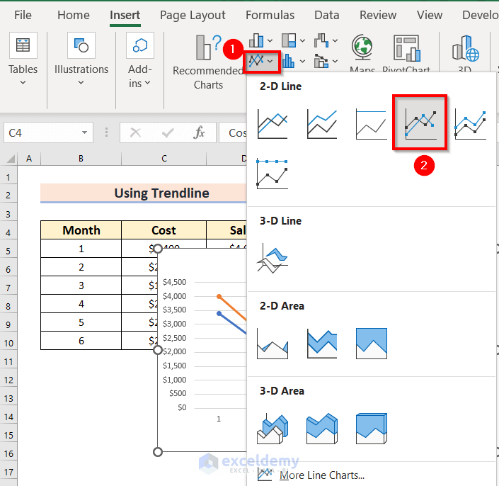
- Select the Charts group and click 2-D Line >>Select a feature (Line with Markers, here).
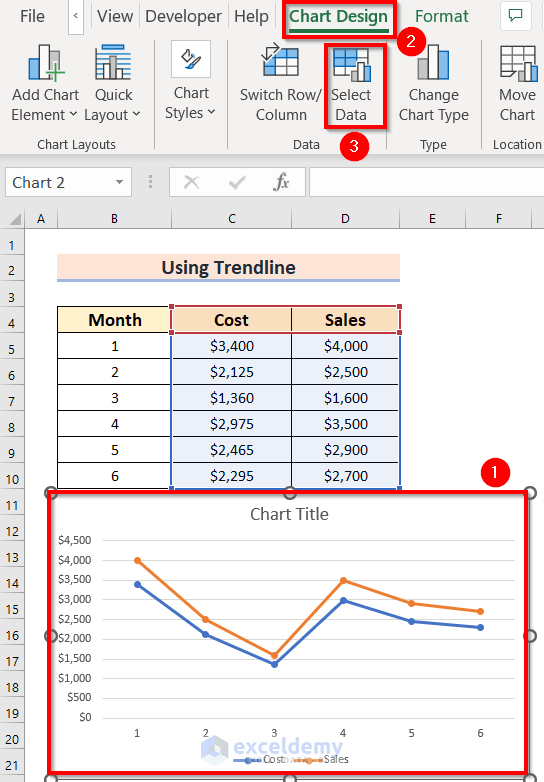
- Select the chart.
- In Chart Design >> choose Select Data.
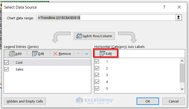
In the Select Data Source dialog box:
- Select Edit to include Axis Labels.
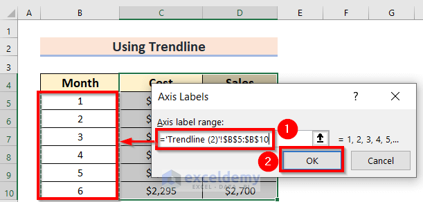
In the Axis Labels dialog box:
- Select the Axis label range. Here, B5:B10.
- Click OK.
- Click OK on the Select Data Source box.
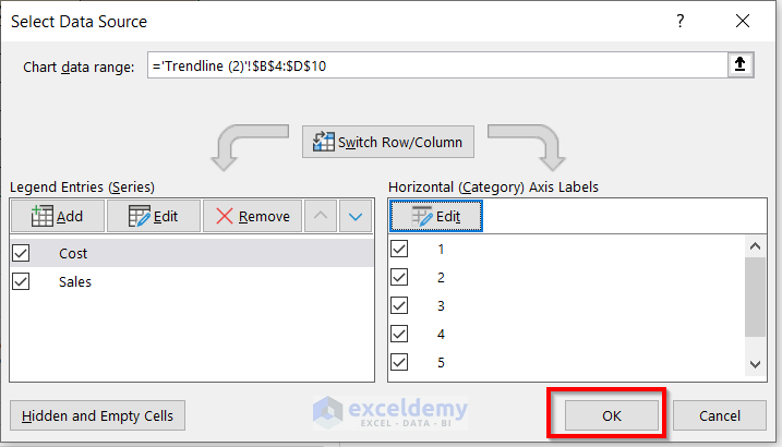
The data chart will be displayed.
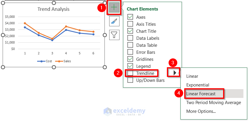
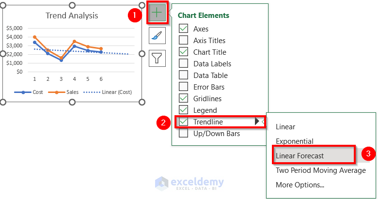
- Click the + icon.
- In Trendline >> select Linear Forecast.
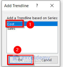
In the Add Trendline dialog box:
- Select Cost.
- Click OK.
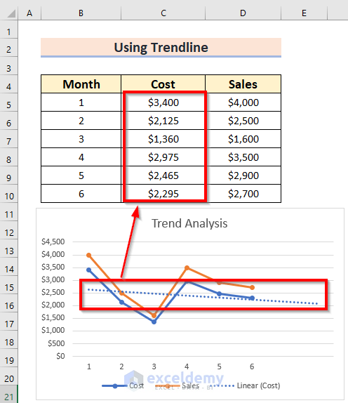
The forecast Trendline for Cost is displayed.
Apply the same process to find the Trendline for Sales.
- Click the + icon.
- In Trendline >> select Linear Forecast.
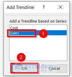
In the Add Trendline dialog box.
- Select Sales.
- Click OK.
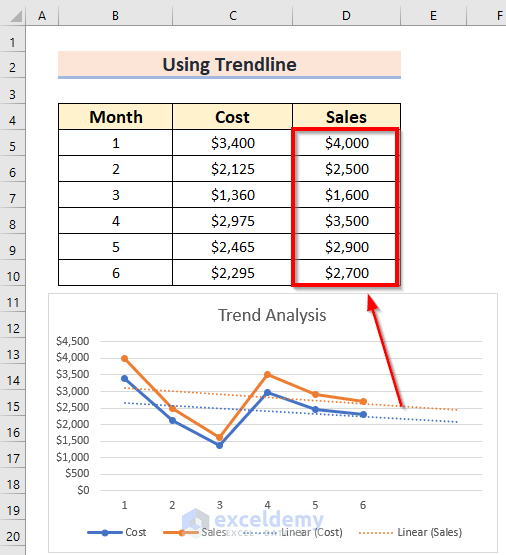
The forecast Trendline for Sales is displayed.
- Click the Trendline you want to format.
- Choose Trendline Options. Here, line width was changed.
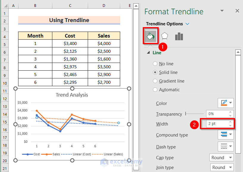
This is the output.
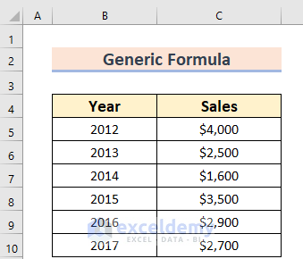
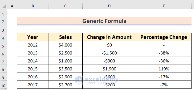
Method 3 – Applying a Generic Formula to Calculate Trend Analysis
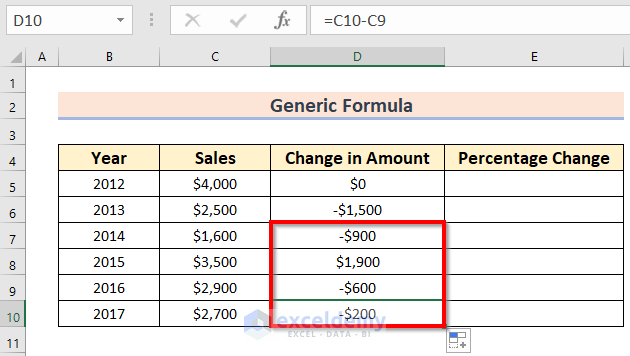
The following dataset contains two columns: Year and Sales.
Steps:
- Select a different cell (D6, here) to calculate the Change in Amount.
- Enter this formula.
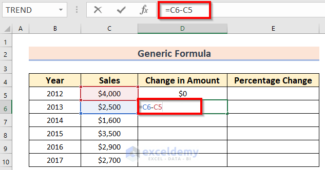
In this formula a simple subtraction (current year 2013- previous year 2012) is applied to get the Change in Amount.
- Press ENTER to see the value in the Change in Amount column.
- Drag the Fill Handle to AutoFill the rest of the cells (D7:D10).
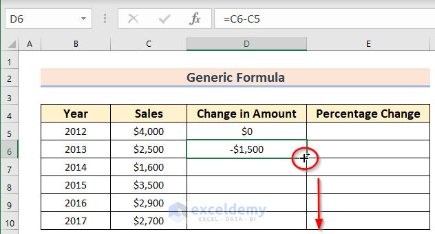
This is the output.
To see the Percentage Change:
- Select a different cell (E6, here) to calculate the Percentage Change.
- Enter this formula.
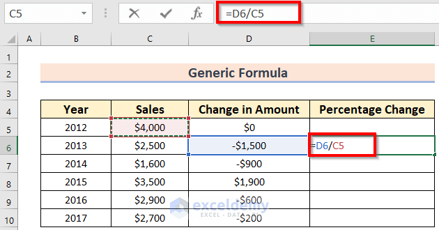
In this formula, a simple division is applied (Change in Amount by the previous year 2012) to get the Percentage Change.
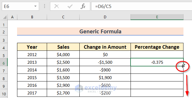
- Press ENTER to see the value in the Percentage Change column.
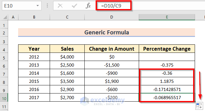
- Drag the Fill Handle to AutoFill the rest of the cells (E7:E10).
This is the output.
- Select the range E5:E10.
- In the Home tab >> select Number and choose Percentage %.
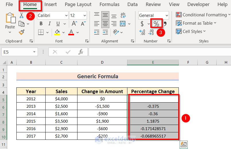
The result is displayed in Percentage.
Calculating Trend Analysis for Multiple Sets of Variables
Steps:
- Select a different cell (E5, here) to calculate the Trend analysis.
- Enter this formula.
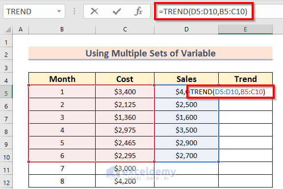
TREND will return a value in a linear way with the given points using the least square method. In this function,
-
- D5:D10 is the known dependent variable, y.
- B5:C10 is the known independent variable, x.
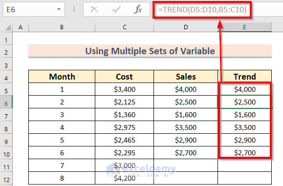
- Press ENTER.
This is the output.
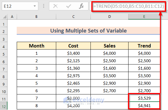
To forecast the Sales for the months of July and August:
- Select a different cell (E11, here) to calculate the Trend analysis of the forecast value.
- Enter this formula.
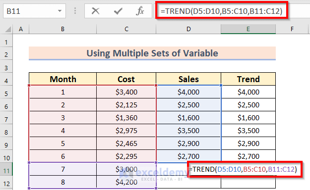
-
- D5:D10 is the known dependent variable, y.
- B5:C10 is the known independent variable, x.
- B11:C12 is the new independent variable, x.
- Press ENTER.
This is the output.
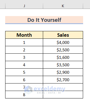
Practice Section
Now, you can practice.
Download Practice Workbook
You can download the practice workbook here:
Related Articles
- How to Make a Polynomial Trendline in Excel
- How to Draw Best Fit Line in Excel
- How to Insert Trendline in an Excel Cell
- How to Create Trend Chart in Excel
- How to Create Monthly Trend Chart in Excel
- How to Calculate Trend Percentage in Excel
<< Go Back To Trendline in Excel | Excel Charts | Learn Excel
Get FREE Advanced Excel Exercises with Solutions!
