How to Find Unknown Value on Excel Graph: 4 Easy Methods

Method 1 – Using TREND Function

Steps:

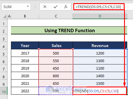
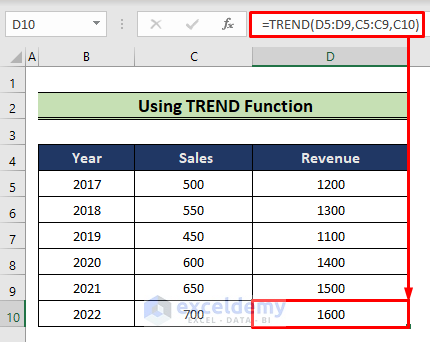
• Select the D10 cell and write the following formula,

• Hit Enter.

• Have our unknown value and can plot it.

Method 2 – Applying Trendline Equation

Steps:

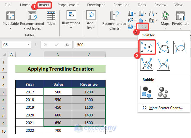
• Select the cells containing the known X and Y
• The cells are in the range (C5:D9).
• Go to the Insert tab in the ribbon.
• Choose the Insert Scatter(X,Y) or Bubble Chart command.
• From the drop-down select a scatter plot.
• A chart will be plotted.

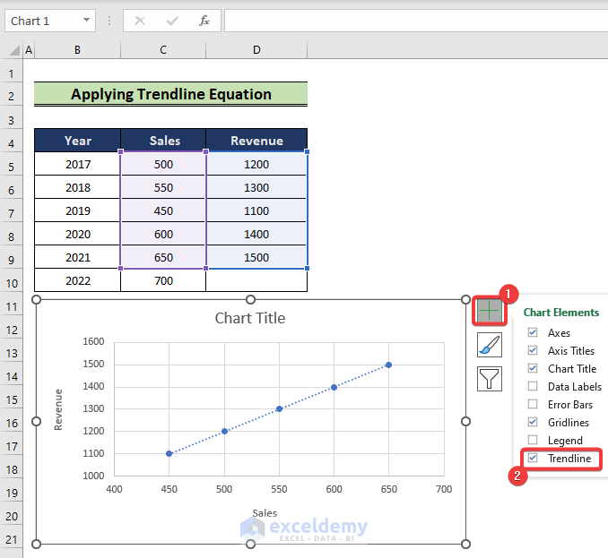
• Click the “Plus” sign to the right of the chart.
• Add a trendline by checking the Trendline box.
• Excel will add a trendline to the plot.

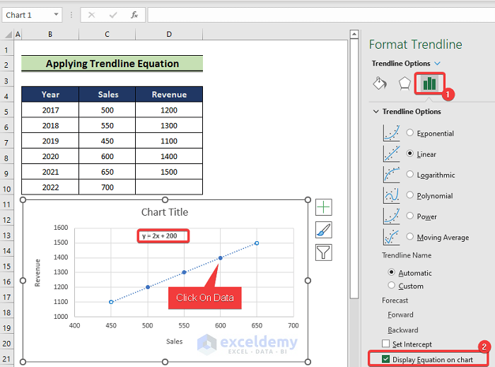
• Select any of the data points.
• From there go to the Trendline Options.
• Check the “Display Equation on chart” box.
• The equation of the chart will be shown on the screen.

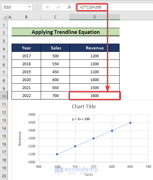
• Replicate the trendline formula in the D10 cell as follows,

• Hit Enter.

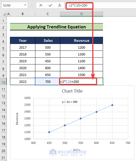
• We will have an unknown value.

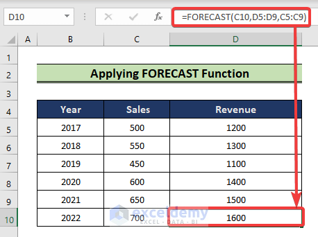
Method 3 – Applying FORECAST Function.

Steps:

• Select the D10 cell and write the following formula,

• Hit  Enter.

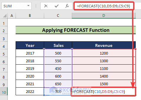
• Have the unknown value and can plot it on the graph.

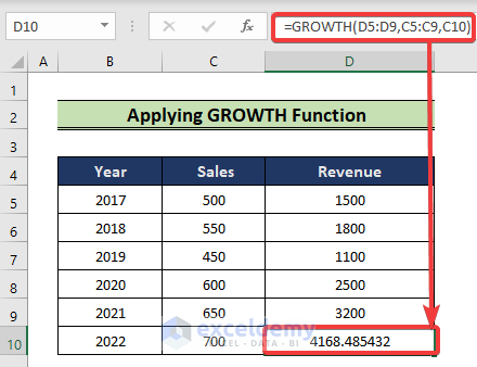
Method 4 – Using GROWTH Function

Steps:

• Start with, choose the D10 cell and write the following formula,

• Press Enter.

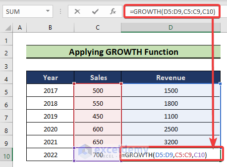
• Get the unknown value and plot it on the graph.

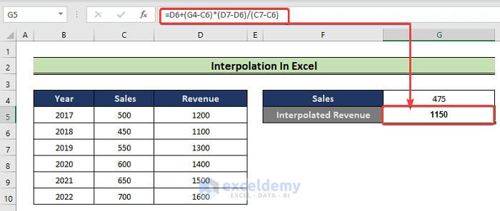
How to Interpolate in Excel

Steps:

• Choose the G5 cell and write the following formula,

• Hit  Enter.

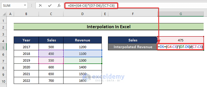
• Get the interpolated value.

Download Practice Workbook

You can download the practice workbook from here.

Related Articles

• How to Add a Trendline to a Stacked Bar Chart in Excel
• How to Extend Trendline in Excel
• How to Exclude Data Points from Trendline in Excel
• [Solved]: Trendline Option Not Showing in Excel
• How to Add Trendline in Excel Online
• How to Show Equation in Excel Graph

<< Go Back To Trendline in Excel | Excel Charts | Learn Excel