How to Fix the Trendline Option Not Showing in Excel

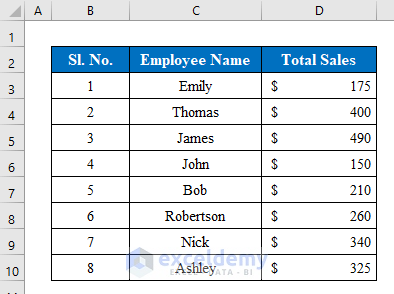
In the below dataset there are Employee Names and their Total Sales volume. We will insert different charts and show you the reasons and solutions for the trendline option not showing in Excel.

The Trendline Option Not Showing Inside a 3D-Chart in Excel

Steps:

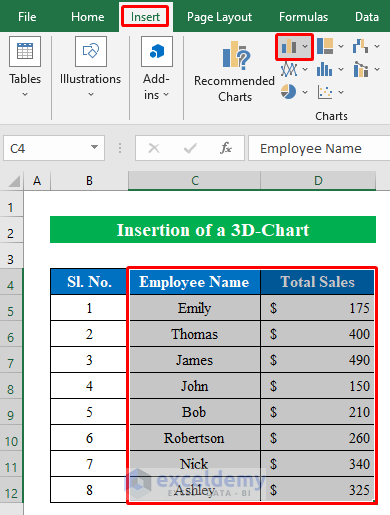
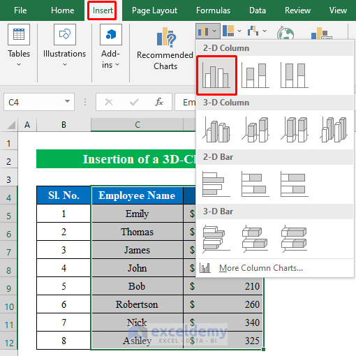
• Choose data from the table that you want to add to the chart. Here, I have selected cells (C4:D12).
• Go to “Charts” from the “Insert” tab.

• From the drop-down list choose a “3-D Clustered Column” chart.

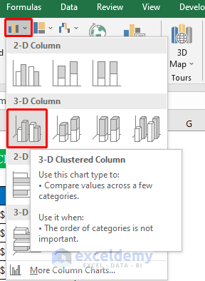
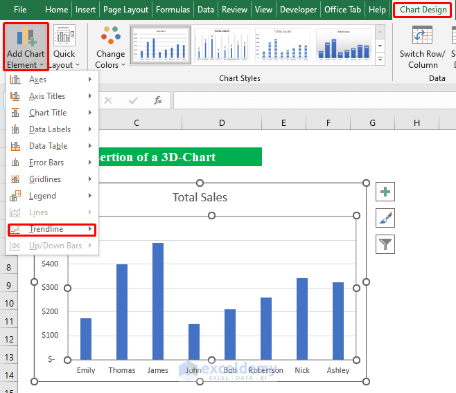
• We get a 3-D chart.
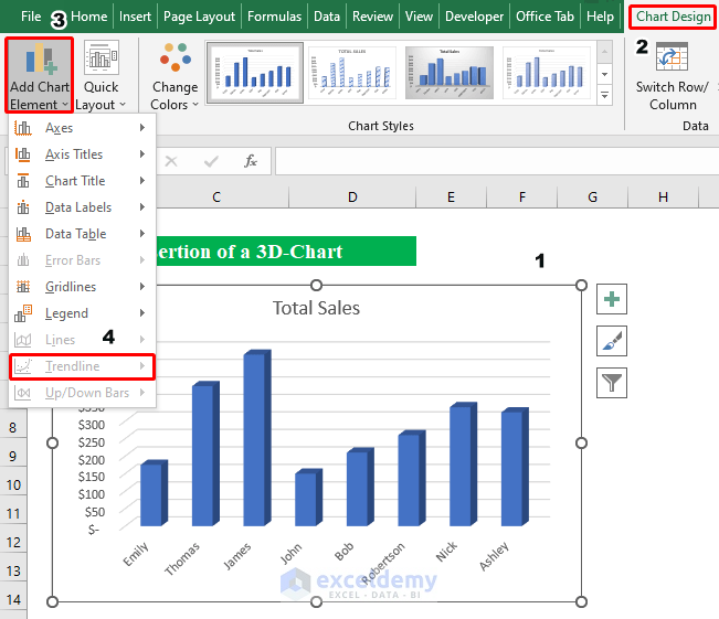
• Go to the “Chart Design” option and open the “Add Chart Element” list.
• You will see the “Trendline” option is not visible.

Solution: Convert the 3D-Chart into a 2D-Chart

Steps:

• Select data from the table.
• Click the “2-D column” from the “Insert” tab.

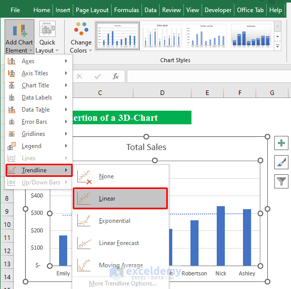
• Open the drop-down list from the “Add Chart Element” list.
• You will get the Trendline option from the list.
• Click the “Trendline” to insert a line inside the chart.

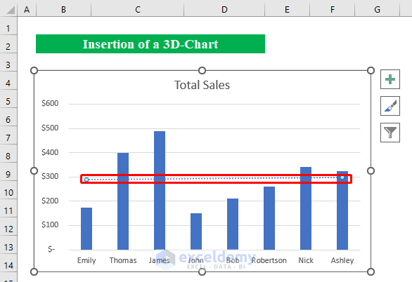
• You can choose from different types of trendlines. Here, I have selected “Linear.”

• We will get our desired result inside the chart just by changing the chart type.

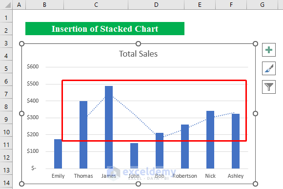
An Excel Stacked Chart Making the Trendline Option Greyed-Out

Steps:

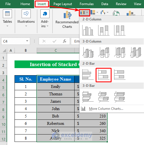
• Select the data from the spreadsheet.
• Go to Insert > 2-D Bar Chart.

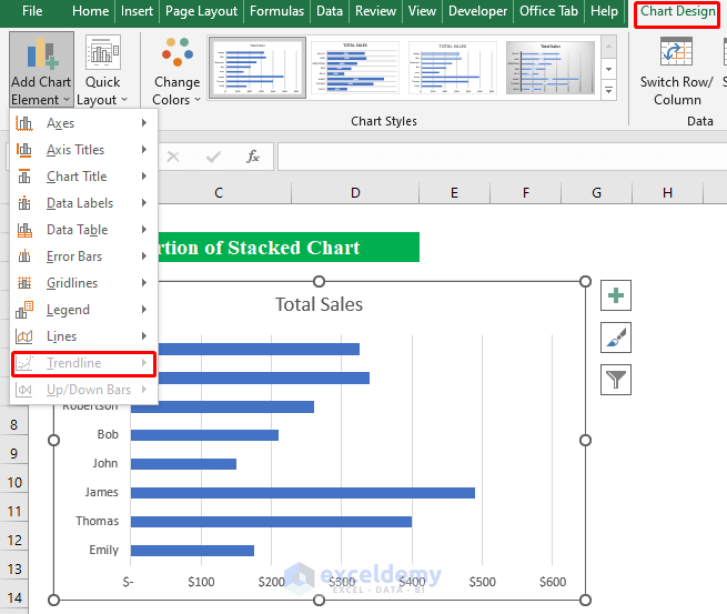
• Open the “Add Chart Element” but the “Trendline” is greyed-out.

Solution: Change the Chart Type

Steps:

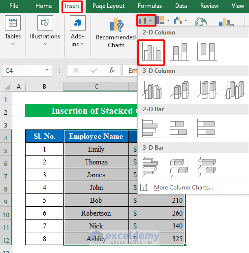
• Choose data from the table and select a 2-D column chart from the “Insert” tab.

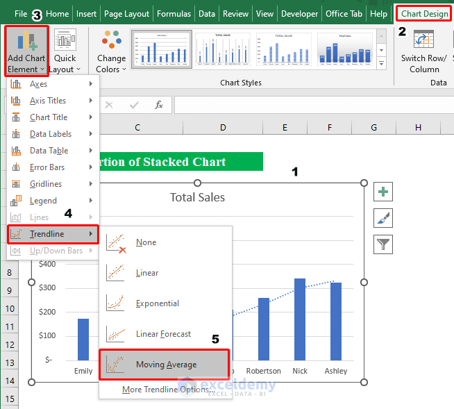
• In this 2-D column chart, you can get the “Trendline” from the “Chart Design” option.
• I have chosen the “Moving Average” trendline. You can select any trendline of your choice.

• We will get the Trendline inside the chart.

Read More: How to Add a Trendline to a Stacked Bar Chart in Excel

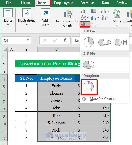
A Pie or Doughnut Chart Disabling the Trendline Option

Steps:

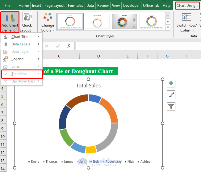
• Create a doughnut chart from the “Insert” tab choosing data from the dataset.

• When selecting the chart, if you go to “Add Chart Elements,” you will see the “Trendline” option is not available.

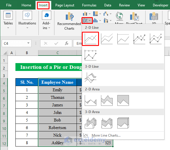
Solution: Use a Different Chart

Steps:

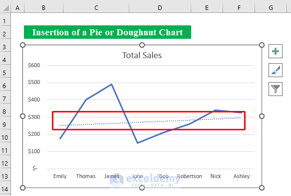
• Create a “2-D line chart” by selecting the data.

• Draw a “Trendline” inside the chart.
• Click “Exponential” from the “Trendline” list.

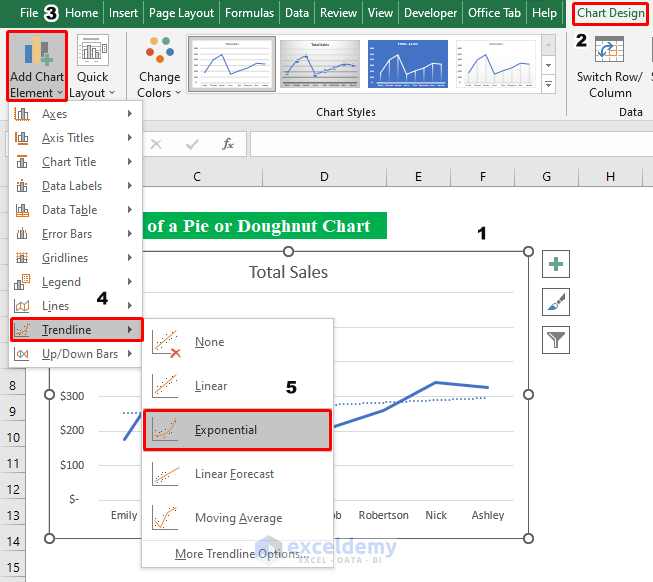
• You will get the trendline inside the chart.

Things to Remember

• You can also change the trendline format from the “Chart Elements” option.
• In a chart, a trend line must be associated with at least three highs or lows for it to be considered genuine.

Download the Practice Workbook

Download this workbook to practice.

Related Articles

• How to Add Trendline Equation in Excel
• How to Find Unknown Value on Excel Graph
• How to Extend Trendline in Excel
• How to Exclude Data Points from Trendline in Excel
• How to Add Trendline in Excel Online

<< Go Back To Trendline in Excel | Excel Charts | Learn Excel