How to Add a Trendline to a Stacked Bar Chart in Excel (2 Methods)

Dataset Overview

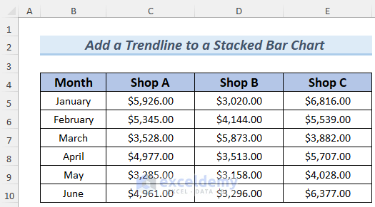
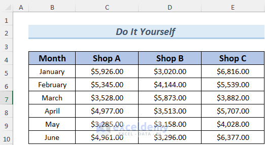
We’ll use the following dataset that contains the sales data of three shops for the first six months of the year:

how to add a trendline to a stacked bar chart in excel

Method 1 – Using Series Lines Feature

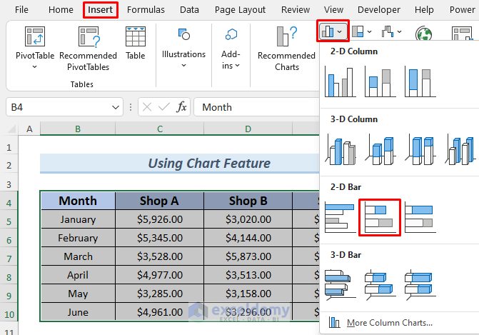
Select the data range (B4:E10) and go to the Insert tab.
Choose 2-D Bar and then select Stacked Bar Chart.

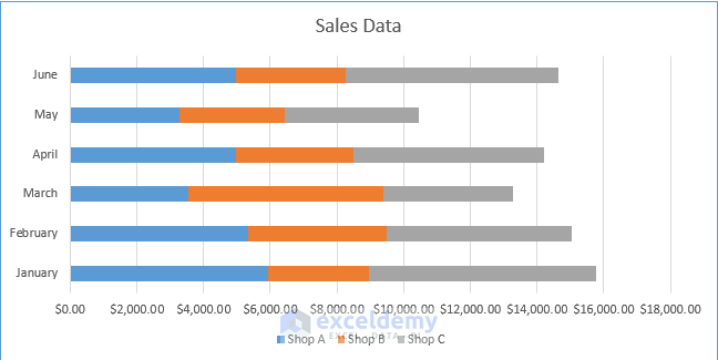
Format the chart as needed (e.g., adjust borders).
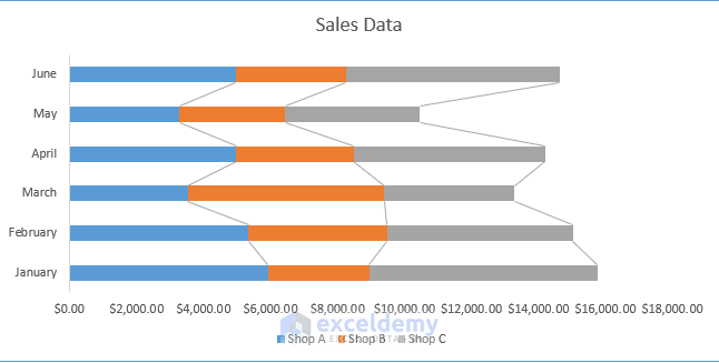
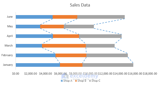
The sales amount of these shops is classified by a particular set of colors: Blue, Red, and Gray are for Shop A, B, and C respectively.

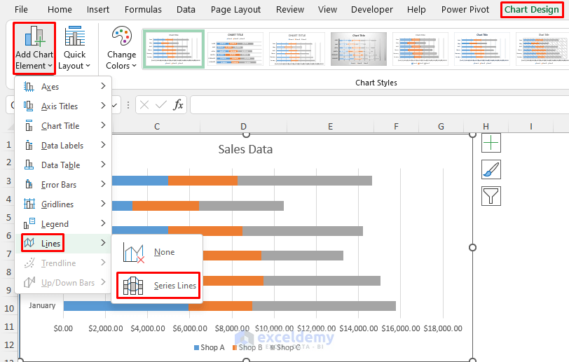
Select the chart and go to Chart Design.
Click Add Chart Element >> Lines >> Series Lines.

The Series Lines in the Stacked Bar Chart will be displayed. The gridlines were removed to improve the visual effect.

Customize the appearance by right-clicking on the series lines and selecting Format Series Lines.

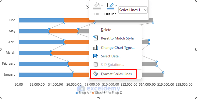
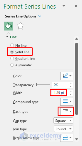
Select the option from the Format Series Lines window to change the appearance of the Series Lines. Select the Solid Line as the Line option, increased the width to 25 pt, and changed the Dash type.

The Stacked Bar Chart looks like the following image:

Result: Your Stacked Bar Chart now includes trendlines created using the Series Lines feature.

Read More: How to Create Trend Chart in Excel

Method 2 – Using VBA (Visual Basic for Applications)

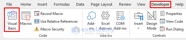
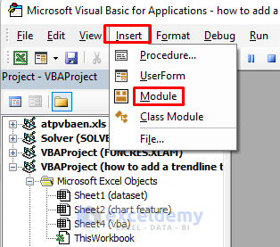
Go to the Developer tab and click Visual Basic.

Insert a new module.

Insert the following code in the module:

Sub StackedBarChartTrendline()
    Range("B4:E10").Select
    ActiveSheet.Shapes.AddChart2(297, xlBarStacked).Select
    ActiveChart.SetSourceData Source:=Range("'vba'!$B$4:$E$10")
    ActiveChart.ChartGroups(1).HasSeriesLines = True
End Sub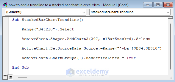

This code uses the Range.Select property and xlBarStacked Enumeration to make a Stacked Bar Chart based on the range B4:E10.

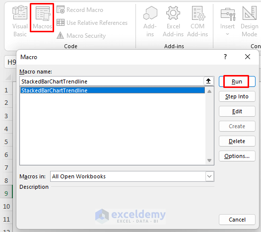
Return to your sheet and execute the macro.

The Stacked Bar Chart will now have series lines acting as trendlines.

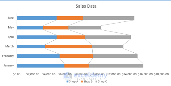
Remember to format these lines as needed, following the procedure described in the previous method. We can consider them as Stacked Trendlines for this chart.