How to Find the Equation of a Trendline in Excel- 5 Steps

What Is Trendline in Excel?

A trendline is a linear or curved line in a graph or chart that defines the general pattern of the selected dataset. It is also referred to as the line of best fit.

To find the equation of a line:

Step 1- Prepare Dataset

Create a dataset with information of Item Name, Sold Items, and Sales amount of 6 types of fruits (here).

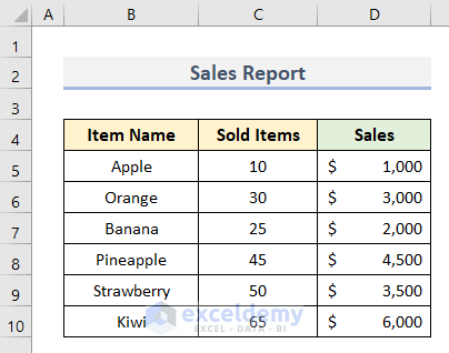
The values in columns C and D act as Y and X axis.

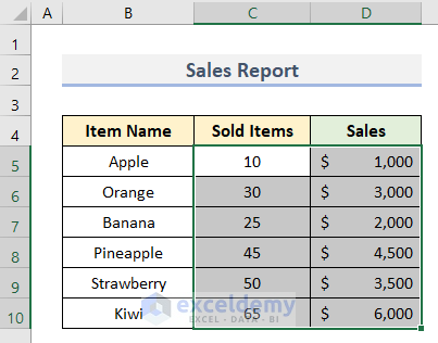
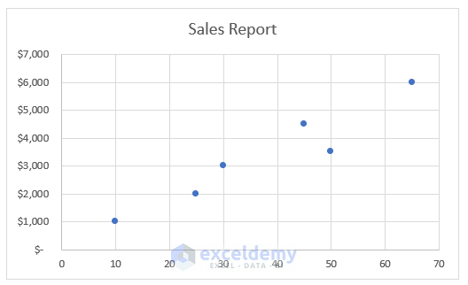
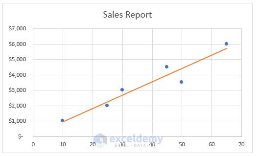
Step 2 – Create a Scatter Chart

• Select C5:D10.

• Go to Insert and select Scatter Chart in Charts.

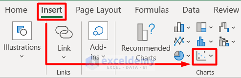
• Choose Scatter.

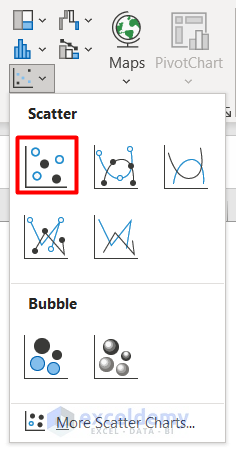
• You will see the chart.

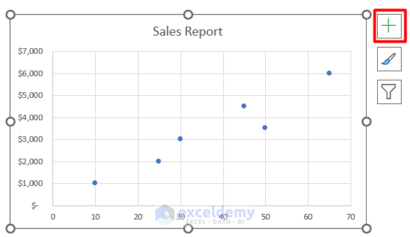
Step 3 – Add a Trendline to the Chart

• Select the chart.
• Click the Plus (+) icon to open Chart Elements.

• Check Trendline.

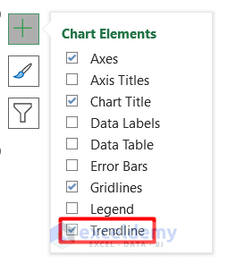
• You will see a trendline.

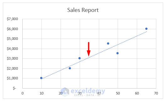
• Format the trendline:

Read More: How to Add a Trendline to a Stacked Bar Chart in Excel

Step 4 – Find the Equation of the Line

• Select the line.
• Right-click it and choose Format Trendline.

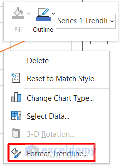
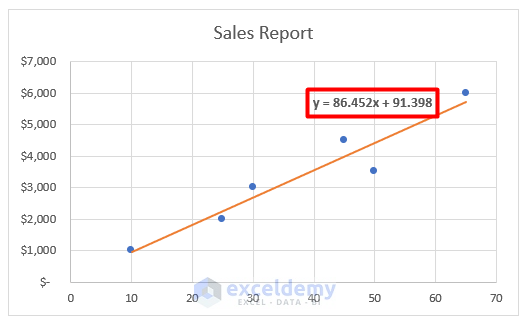
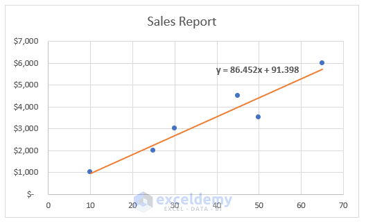
• In the Format Trendline panel, check Display Equation on chart.

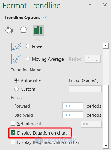
• The equation is displayed beside the line.

Read More: How to Show Equation in Excel Graph

Step 5 – Add Decimal Places to the Equation

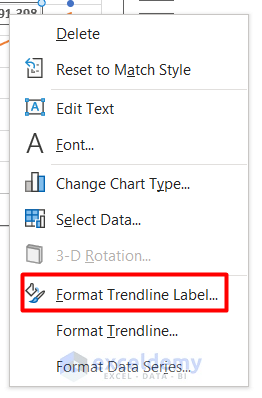
• Select the trendline again.
• Right-click it and select Format Trendline Label.

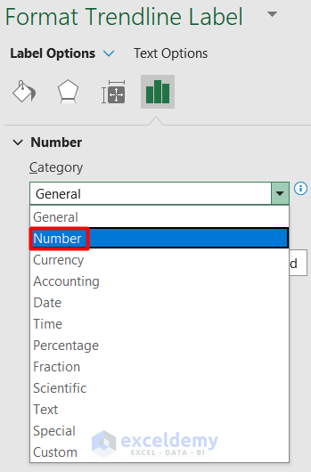
• Select Number in Category.

• Enter a value in Decimal places.

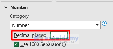
• Decimal points are displayed in the line equation.

Read More: How to Create Equation from Data Points in Excel

How to Find the Slope of Line Equation in Excel

To get the slope of the equation, use the SLOPE function.

• Select C12.
• Enter this formula.

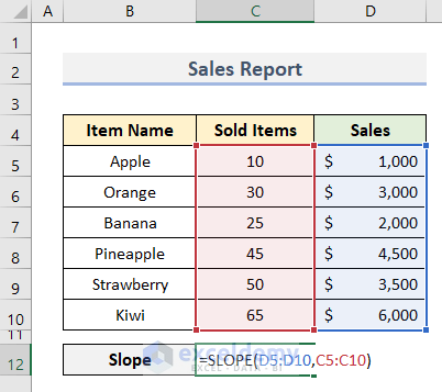
• Press Enter.
• The value of the slope for the line is displayed.

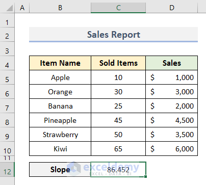
The SLOPE function was used to calculate the change rate between dependent and independent variables. D5:D10 defined the dependent data points on the Y axis. C5:C10 acts as the independent data points plotted on the X-axis.

Download Practice Workbook

Download the sample file.

Related Articles

• How to Find the Equation of a Trendline in Excel
• How to Use Trendline Equation in Excel
• How to Find Slope of Trendline in Excel
• How to Find Unknown Value on Excel Graph
• How to Find Intersection of Two Trend Lines in Excel

<< Go Back To Trendline Equation Excel | Trendline in Excel | Excel Charts | Learn Excel