How to Use Trendline Equation in Excel: 8 Suitable Examples

Method 1 – Adding Trendline Equation in Excel

Steps:

Select the chart in which you want to add the trendline.
Go to Chart Elements.
Select Trendline.

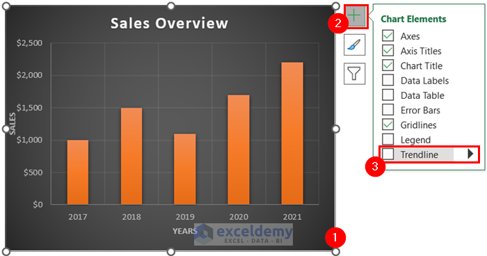
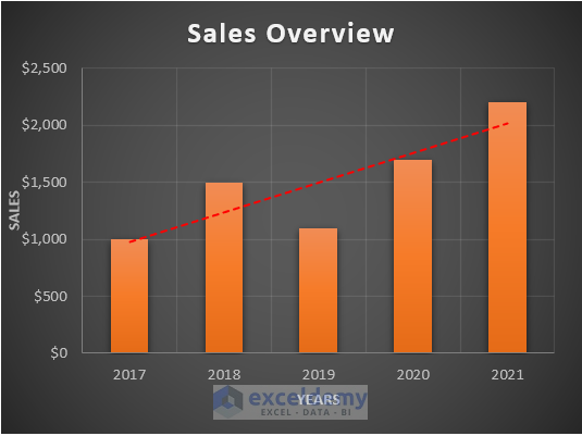
You will see a trendline has been added to your chart.

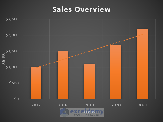
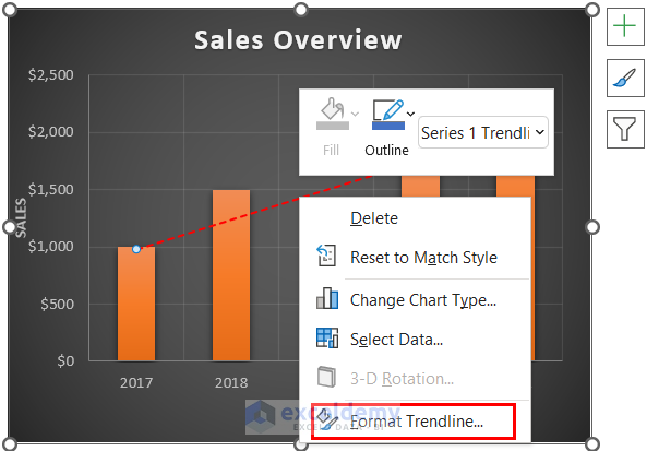
Adding Trendline Equation in Excel

Change the color of the trendline to make it more visible.

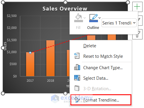
Right-click on the trendline.
Select Format Trendline.

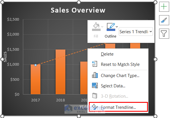
See that the Format Timeline option will appear on the right side of the screen.

Go to Fill & Line.
Select Color.

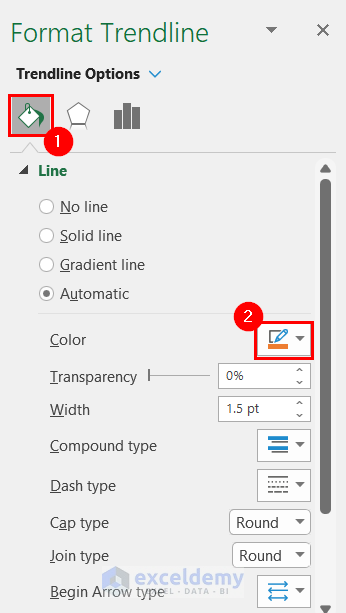
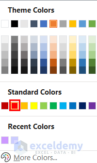
See a list of colors that will appear.

Select the color you want. Here, I selected Red.

See that you have got your desired trendline.

Change the trendline type.

Right-click on the trendline.
Select Format Trendline.

The Format Timeline option will appear on the right side of the screen.

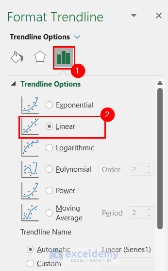
Go to the Trendline Options.
Select the trendline type you want. We kept it linear, which is the default option, but you can select any other option.

Add the trendline equation.

Right-click on the trendline.
Select Format Trendline.

The Format Timeline option will appear on the right side of the screen.

Go to the Trendline Options.
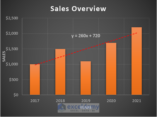
Select Display Equation on chart.

See the trendline equation on the chart.

Method 2 – Using Trendline Equation in Excel to Forecast Data

Steps:

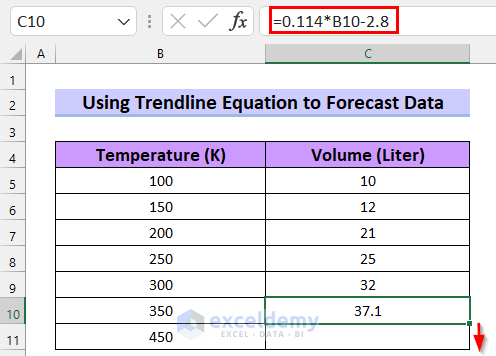
Select the cell where you want to forecast the data. We selected cell C10.
In cell C10 write the following formula.

=0.114*B10-2.8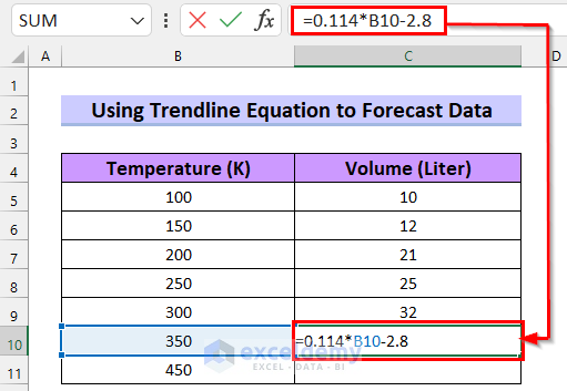

We used the trendline equation from the chart. I took B10 as X. The formula will return the Y value.

Press ENTER to get the Y.

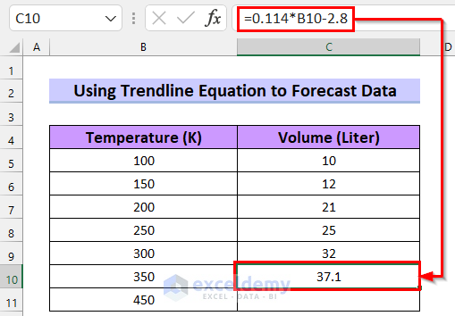
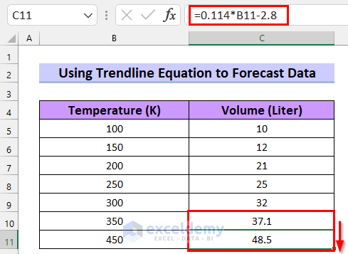
Drag the Fill Handle to copy the formula.

See that you have got your forecasted data using the trendline equation in Excel.

Method 3 – Using Trendline Equation in Excel to Get Values for Any Given X

Steps:

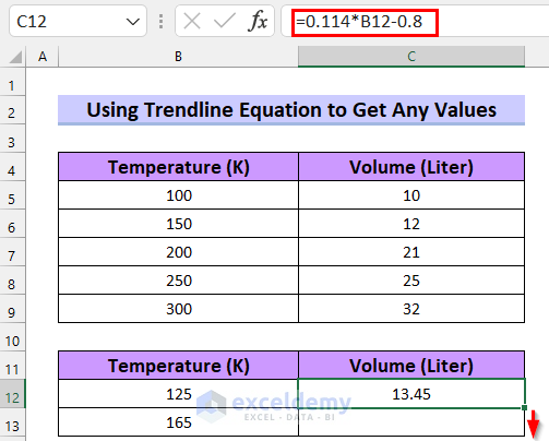
Select the cell where you want to get the Y value for a given X. We selected cell C12.
In cell C12 write the following formula.

=0.114*B12-0.8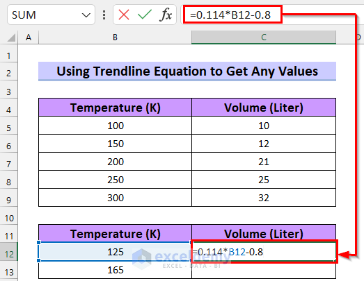

We used the trendline equation from the chart. We took B12 as X. Now, the formula will return the Y value.

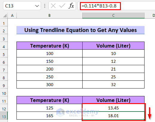
Press ENTER to get the Y.

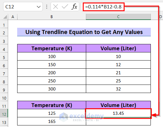
Drag the Fill Handle to copy the formula.

See that you have your Y values for any given X using the trendline equation in Excel.

Method 4 – Inserting Linear Trendline Equation to Find Slope and Intercept

Steps:

Select the cell where you want to calculate the Slope. We selected cell G5.
In cell G5 write the following formula.

=SLOPE(C5:C9,B5:B9)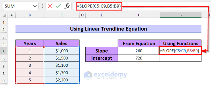

In the SLOPE function, I selected C5:C9 as known_ys and B5:B9 as known_xs. This function will return the value of the Slope for the dataset.

Press ENTER to get the value of the Slope.

Calculate the Intercept.

Select the cell where you want to calculate the Intercept. We selected cell G6.
In cell G6 write the following formula.

=INTERCEPT(C5:C9,B5:B9)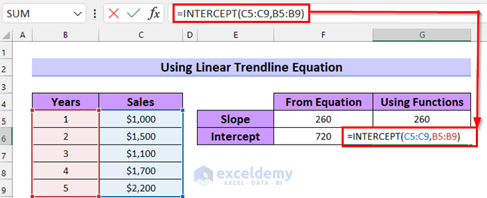

In the INTERCEPT function, I selected C5:C9 as known_ys and B5:B9 as known_xs. This function will return the value of the Intercept for the dataset.

Press ENTER to get the value of the Intercept.

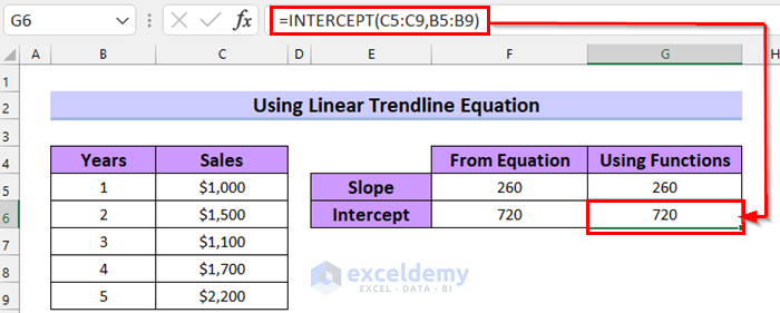
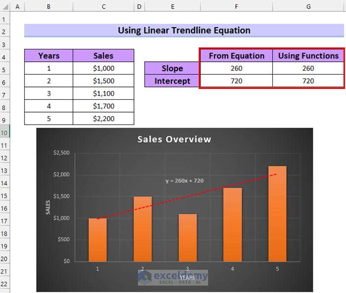
See that the Slope and Intercept values from the equation match the values we got using functions. This means the values from the trendline equation are correct.

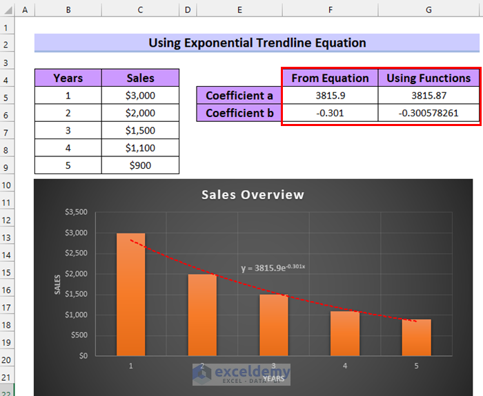
Method 5 – Using Exponential Trendline Equation in Excel to Find the Coefficients

Steps:

Select the cell where you want to calculate the Coefficient a. We selected cell G5.
In cell G5 write the following formula.

=EXP(INDEX(LINEST(LN(C5:C9),B5:B9),1,2))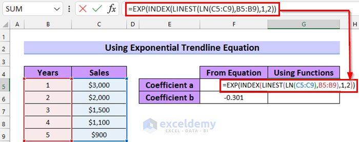

Formula Breakdown

Here, in the EXP function, used the INDEX function as a number that will return the value from a range.
Now, in the INDEX function, used the LINEST function as array 1 as row_num, and 2 as column_num.
Next, In the LINEST function, selected LN(C5:C9) as known_ys the LN function will return the natural logarithm of the given range, and B5:B9 as known_xs.
Finally, the EXP function will return the result of the constant e raised to the power of the number, which will be our coefficient a.

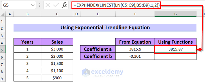
Press ENTER to get the coefficient a.

Calculate Coefficient b.

Select the cell where you want to calculate the Coefficient b. We selected cell G6.
In cell G6 write the following formula.

=INDEX(LINEST(LN(C5:C9),B5:B9),1)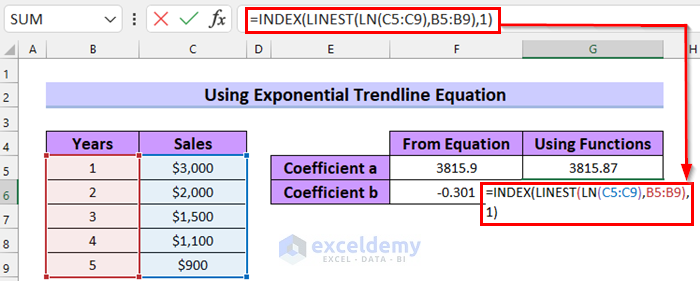

Formula Breakdown

In the INDEX function, I used a LINEST function as array and 1 as row_num.
In the LINEST function, I selected LN(C5:C9) as known_ys which will return the natural logarithm of the given range, and B5:B9 as known_xs.
The INDEX function will return the value from the table which will be Coefficient b.

Press ENTER to get the Coefficient b.

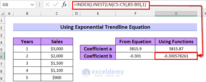
See that the values of Coefficient a and Coefficient b from the equation match the values we got using functions. This means the values from the trendline equation are correct.

Method 6 – Applying Logarithmic Trendline Equation in Excel

Steps:

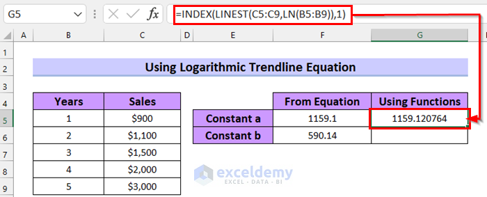
Select the cell where you want to calculate the Constant a. We selected cell G5.
In cell G5 write the following formula.

=INDEX(LINEST(C5:C9,LN(B5:B9)),1)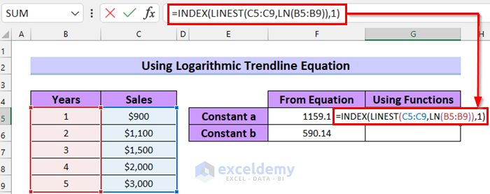

Formula Breakdown

In the INDEX function, used a LINEST function as array and 1 as row_num.
In the LINEST function, selected C5:C9 as known_ys, and LN(B5:B9) as known_xs which will return the natural logarithm of the given range.
The INDEX function will return the value from the table will be Constant a.

Press ENTER to get the Constant a.

Calculate Constant b.

Select the cell where you want to calculate the Constant b. Here, I selected cell G6.
In cell G6 write the following formula.

=INDEX(LINEST(C5:C9,LN(B5:B9)),1,2)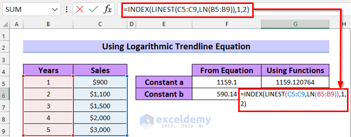

Formula Breakdown

In the INDEX function, used a LINEST function as array and 1 as row_num and 2 as column_num.
In the LINEST function, selected C5:C9 as known_ys, and LN(B5:B9) as known_xs will return the natural logarithm of the given range.
The INDEX function will return the value from the table will be Constant b.

Press ENTER to get the Constant b.

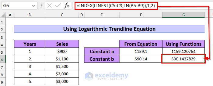
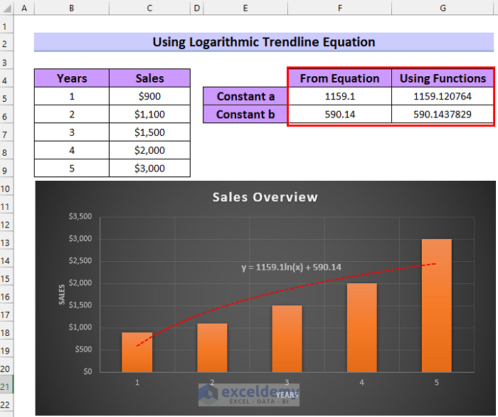
See that the values of Constant a and Constant b from the equation match the values we got using functions. This means the values from the trendline equation are correct.

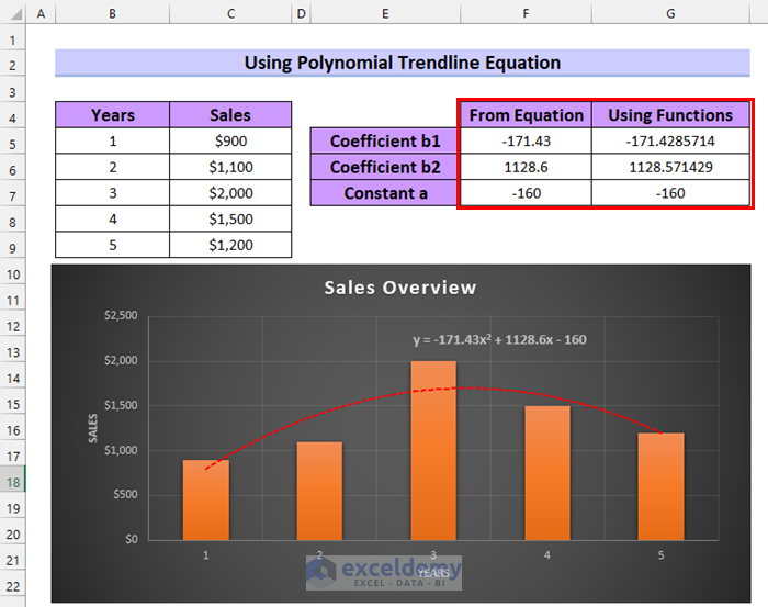
Method 7 – Using Polynomial Trendline Equation in Excel

Steps:

Select the cell where you want to calculate the Coefficient b1. We selected cell G5.
In cell G5 write the following formula.

=INDEX(LINEST(C5:C9,B5:B9^{1,2}),1)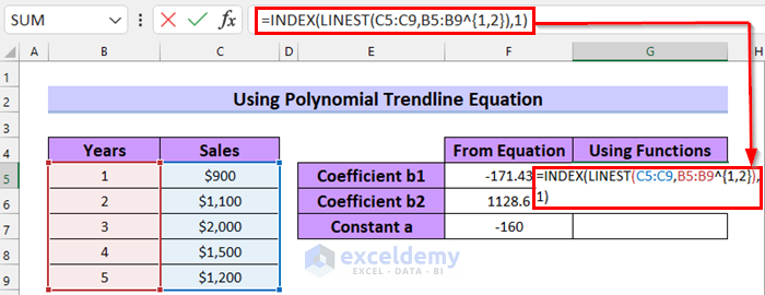

Formula Breakdown

In the INDEX function, I used a LINEST function as array and 1 as row_num.
In the LINEST function, I selected C5:C9 as known_ys, and B5:B9^{1,2} as known_xs which will raise the range B5:B9 to the power of {1,2}.
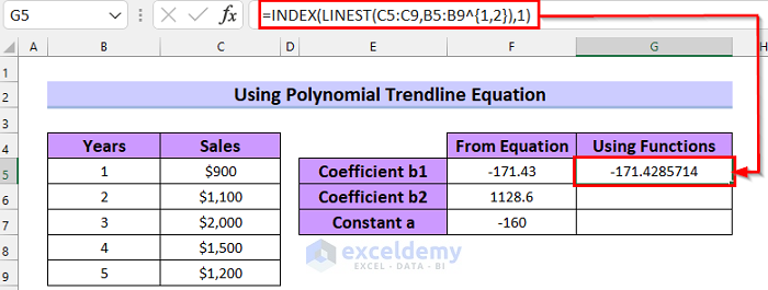
The INDEX function will return the value from the table will be Coefficient b1.

Press ENTER to get Coefficient b1.

Calculate Coefficient b2.

Select the cell where you want to calculate the Coefficient b2. Here, I selected cell G6.
In cell G6 write the following formula.

=INDEX(LINEST(C5:C9,B5:B9^{1,2}),1,2)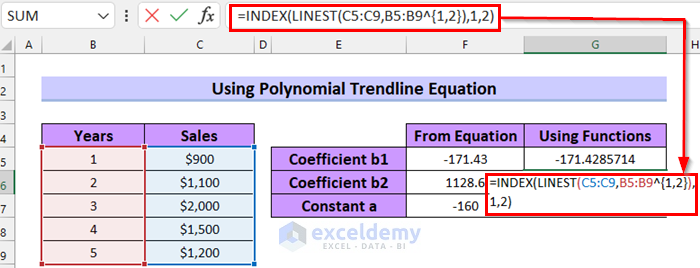

Formula Breakdown

In the INDEX function, used a LINEST function as array, 1 as row_num and, 2 as column_num.
In the LINEST function, selected C5:C9 as known_ys, and B5:B9^{1,2} as known_xs which will raise the range B5:B9 to the power of {1,2}.
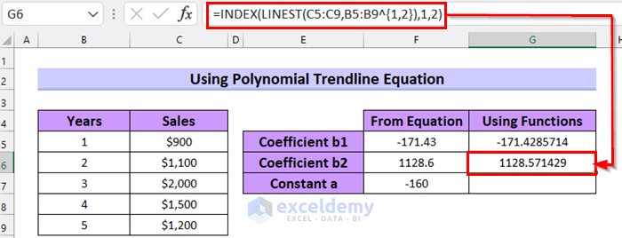
The INDEX function will return the value from the table will be Coefficient b2.

Press ENTER to get Coefficient b2.

Calculate Constant a.

Select the cell where you want to calculate the Constant a. We selected cell G7.
In cell G7 write the following formula.

=INDEX(LINEST(C5:C9,B5:B9^{1,2}),1,3)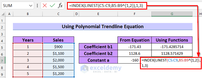

Formula Breakdown

In the INDEX function, used a LINEST function as array, 1 as row_num and, 3 as column_num.
In the LINEST function, selected C5:C9 as known_ys, and B5:B9^{1,2} as known_xs which will raise the range B5:B9 to the power of {1,2}.
The INDEX function will return the value from the table which will be Constant a.

Press ENTER to get Constant a.

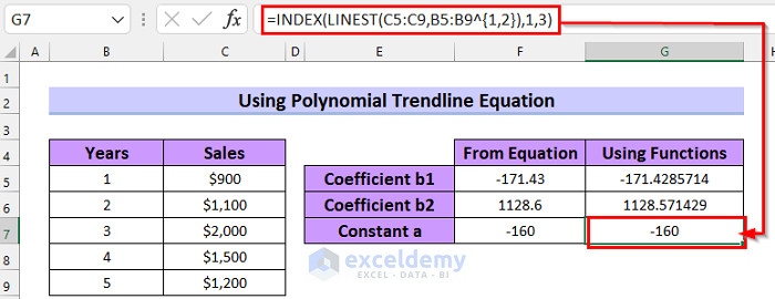
See that the values of Coefficient b1, Coefficient b2, and Constant a from the equation match the values that we got using functions. This means the values from the trendline equation are correct.

Method 8 – Using Power Trendline Equation in Excel

Steps:

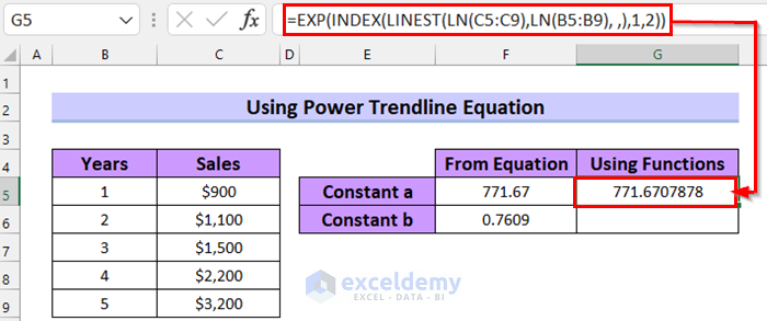
Select the cell where you want to calculate the Constant a. We selected cell G5.
In cell G5 write the following formula.

=EXP(INDEX(LINEST(LN(C5:C9),LN(B5:B9), ,),1,2))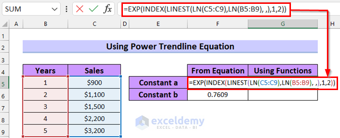

Formula Breakdown

In the EXP function, used an INDEX function as a number that will return the value from a range.
In the INDEX function, used a LINEST function as an array and 1 as row_num, and 2 as column_num.
In the LINEST function, selected LN(C5:C9) as known_ys which will return the natural logarithm of the given range, and LN(B5:B9) as known_xs which will return the natural logarithm of the given range, and left const and stats
The EXP function will return the result of the constant e raised to the power of the number which will be our Constant a.

Press ENTER to get the Constant a.

Now, I will calculate Constant b.

Select the cell where you want to calculate the Constant a. We selected cell G6.
In cell G6 write the following formula.

=INDEX(LINEST(LN(C5:C9),LN(B5:B9),,),1)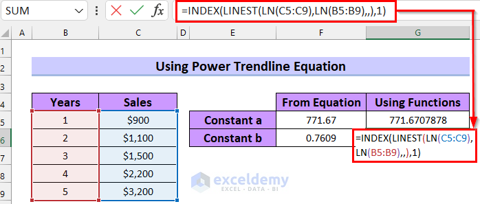

Formula Breakdown

In the INDEX function, used a LINEST function as an array and 1 as row_num.
In the LINEST function, selected LN(C5:C9) as known_ys which will return the natural logarithm of the given range, and LN(B5:B9) as known_xs which will also return the natural logarithm of the given range, and left const and stats
The INDEX function will return the value from the table which will be Constant b.

Press ENTER to get the Constant b.

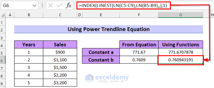
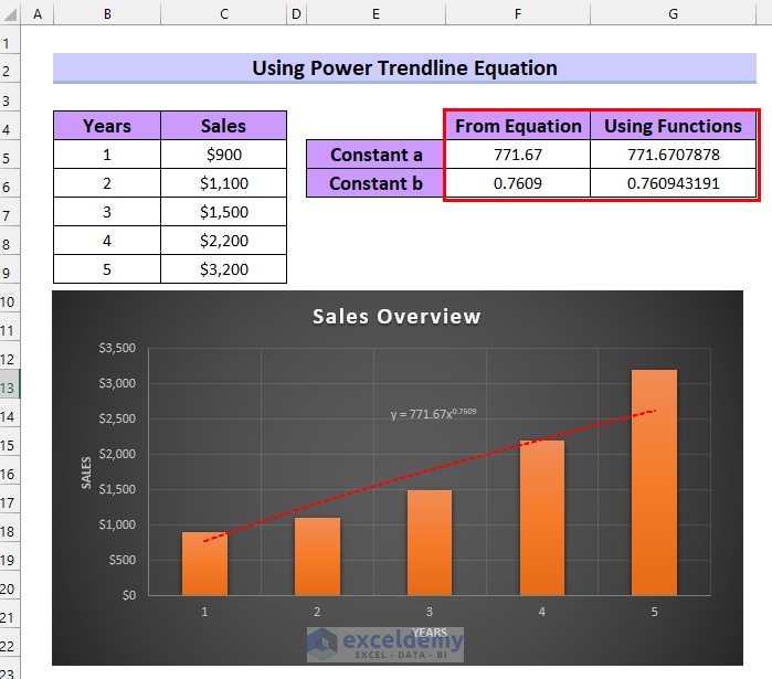
See that the values of Constant a and Constant b from the equation match the values that we got using functions. This means the values from the trendline equation are correct.