We can perform employee scheduling algorithm in Excel using the in-built Solver feature. This algorithm is particularly handy when it comes to efficient workforce management for an organization.
We will perform an employee scheduling algorithm for a hospital. First, we have to create a dataset. Then we will create a result outline and insert a suitable formula. And, lastly, we will carry out the analysis with the Solver feature.
Step 1: Necessary Assumptions for Employee Scheduling Algorithm
For conducting the employee scheduling Algorithm, we must make some assumptions.
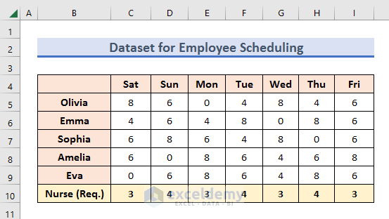
- Let’s take a dataset of five nurses and the number of hours they are willing to work each day. Also, they might not work every day.
- In row number 10, we have put the minimum number of nurses required for each day.
- Now, let’s modify this dataset.
- Create a data table of nurses and set 0 in every cell like the image below.

- This hospital we are working with provides a minimum of two holidays for their employees.
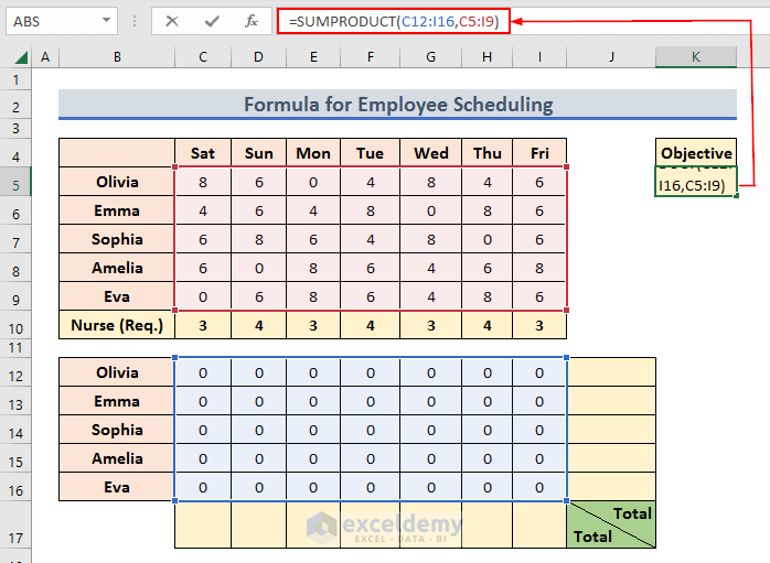
- Add a column and a row like the below image.
- In Column J we will find the total number of days each employee has to work in a week.
- And, Row 17 for the number of employees required each day.
- For this analysis, we also have to insert an Objective box to show the total number of employees working hours in a week.

Read More: How to Create Betting Algorithm in Excel
Step 2: Using SUM AND SUMPRODUCT Functions for Employee Scheduling Algorithm
For this analysis, we have to set some formulas. We are going to use SUMPRODUCT and SUM functions as formulas.
Let’s see them.
We want to find out the maximum possible working hours of the employees in a week.
- So, write the following formula in K5 and press ENTER.
=SUMPRODUCT(C12:I16,C5:I9)
Here,
- C12:I16 = array1
- C5:I9 = array2
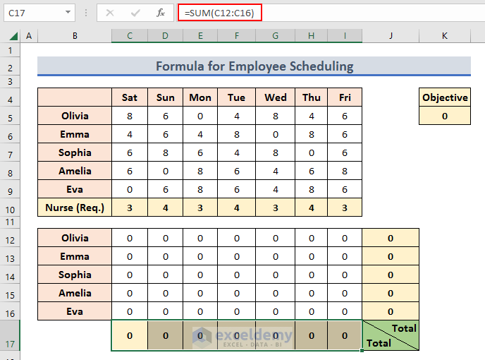
Upon entering the formula, the cell should give 0.

- Now we will use the SUM formula so that we can find the number of days each employee has to work in a week.
- So, write the following formula in J12 and press Enter.
=SUM(C12:I12)
Here,
C12:I12 = Data Range
- Then Hold and Drag the J12 cell downward to copy this formula for all the cells.

- Again, we have to set SUM formula in Row 17 so that we can find the number of nurses working each day.
- So, write the following formula in C17 and press ENTER.
=SUM(C12:C16)
Here,
C12:C16 = Data Range
- Then Hold and Drag the C17 rightward to copy the formula in all the cells.
Thus, our dataset is ready for analysis.
Read More: How to Use Fuzzy LOOKUP Algorithm in Excel
Step 3: Applying the Solver Feature in Excel
Now let’s analyze the dataset with the in-built Solver feature.
- First, go to the Data ribbon and click on the Solver icon.

So, a Solver Parameters window will open.
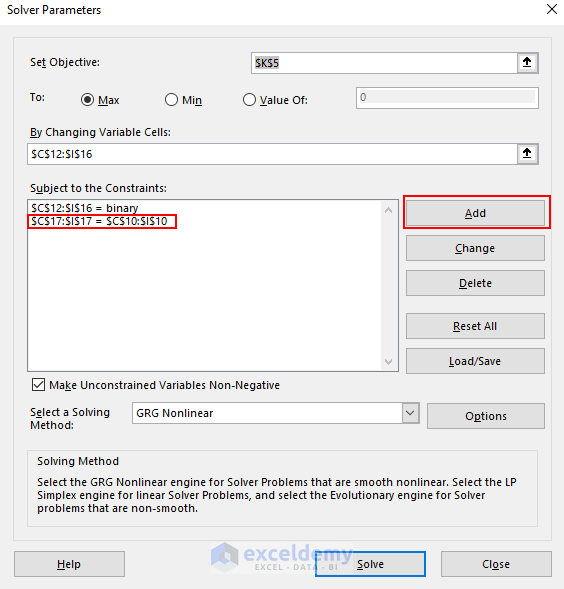
- Now we have to set these solver parameters which is K5 in this case.
- Set the Objective cell in the Set Objective box.
- Keep the To section Max.
- Insert the data array $C$12:$I$16 in the By Changing Variable Cells box.
- Also, we have to set three constraints.
- So, click on Add.

- This constraint is for finding the employee’s working days. We want to know whether an employee works on a given day or not. We want to get the value in binary. 1 will mean they have to work and 0 will mean their holiday.
- So set the Cell Reference to $C$12:$I$16, choose the bin (binary) option from the adjacent box, and press OK.

- The constraint will appear in the Subject to the Constraints box.
- Now, click on Add for another constraint.

- This constraint is for the number of employees required each day which will be equal to the data range C10:I10.
- So, set the data range $C$17:$I$17 in the Cell Reference box.
- Then choose the = (equal) sign in the adjacent box.
- And, set $C$10:$I$10 in the Constraint box and press OK.

- The new constraint will show up in the box.
- Now, we will add the last constraint.
- Click on the Add option.
- This constraint is for setting the maximum working days for each employee in a week.
- So set the data range $J$12:$J$16 in the Cell Reference box.
- Choose the < = (less or equal) sign in the adjacent box
- And lastly set the Constraint to 5 and press OK.

- Thus, we have set all the constraints.
- Now, choose the Simplex LP option from the Select a Solving Method box and click on the Solve button.

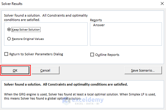
- Doing so, the Solver Results window will open.
- Make sure the Keep Solver Solution is active and press OK.
- Therefore, the solver will give you results.
- The Objective Cell indicates the number of working hours that the organization can get out of its employees.
- The data range C12:I16 shows the working days of each employee in a binary form.
- The data range J12:J16 shows the number of working days in a week for each employee.
- The data range C17:I17 shows the number of nurses assigned on each day.

Download Practice Workbook
You can download and practice this workbook.
Conclusion
Thank you for making it this far. We have shown you how to perform employee scheduling algorithm in Excel. Hope you find the content of this article useful. If there are further queries or suggestions please do mention them in the comment section.
Related Articles
- How to Build Lottery Prediction Algorithm in Excel
- How to Perform Machine Learning in Excel
- How to Use Artificial Intelligence in Excel
- How to Make Decision Tree Algorithm in Excel
- How to Create Rainflow Counting Algorithm in Excel
<< Go Back to Algorithm in Excel | Learn Excel
Get FREE Advanced Excel Exercises with Solutions!
