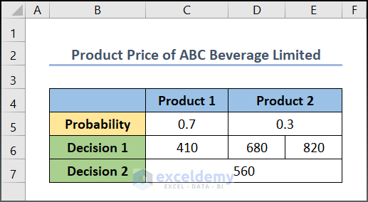
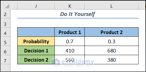
“Product Price of ABC Beverage Limited” is the sample dataset.
Example 1 – Creating a Decision Tree for 4 Events
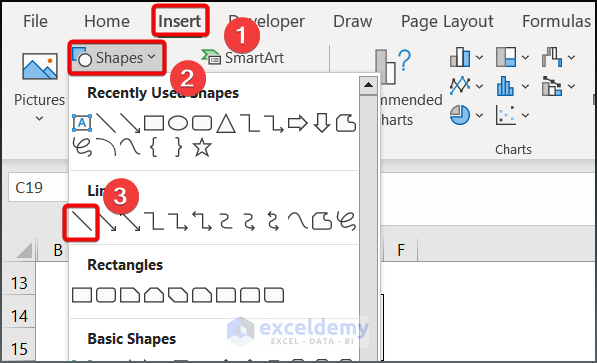
Step 1: Construct Essential Shapes
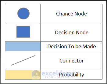
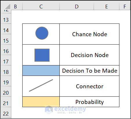
Specific shapes are necessary to draw a decision tree:
- Go to Insert > Shapes >Oval.
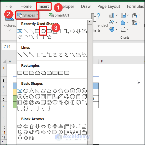
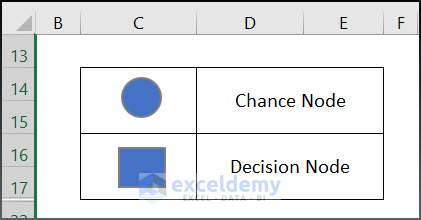
- The oval shape is labelled as Chance Node in the decision tree.
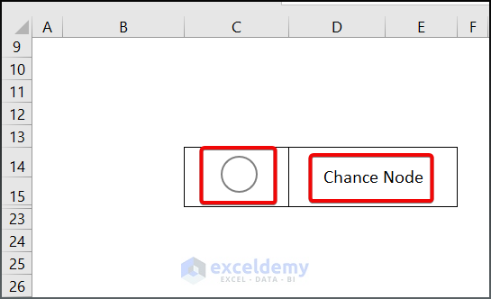
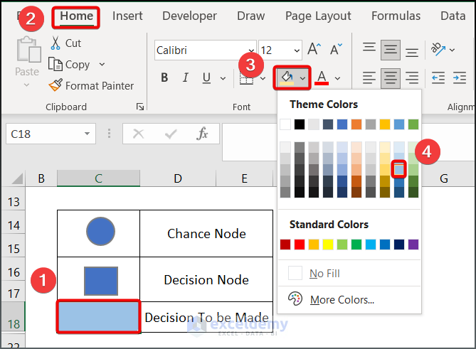
- Choose Blue on the Font ribbon to fill the shape .

- Draw a Rectangular box below the Oval shape and fill it with Blue. Label it Decision Node.
This is the output.
- Fill another cell with Blue accent 5 lighter 40% and label it “Decision to Be Made”.
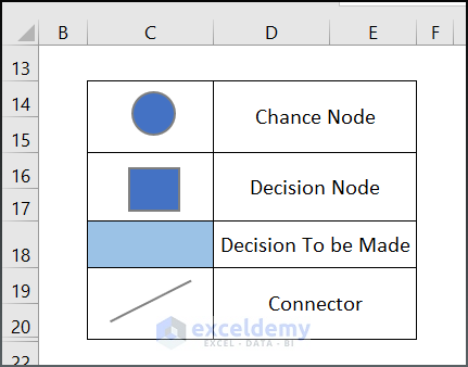
- Go to Insert > Shapes > Line command and draw a line.
This is the output.
- Fill a box with Gold Accent 4, 60% Lighter and label it probability box.

This is the output.
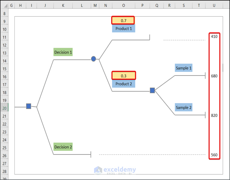
Step 2: Make a Basic Outline of the Tree
- Use CTRL+C & CTRL+V to recreate the figure.

Step 3: Label & Input Values in the Decision Tree
- Input the corresponding value of the dataset in the recreated tree.
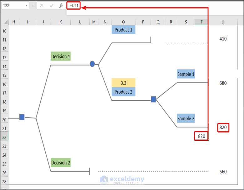
- Enter the following formula in T22 to return event value 820.
=U21
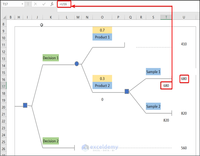
- Enter the following formula to bring the value of U16 into T17.
=U16
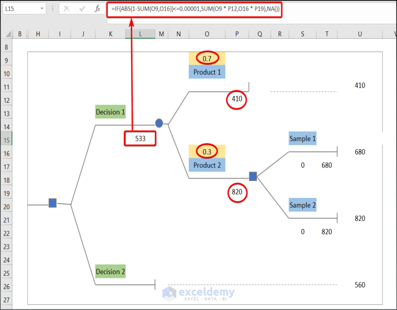
- Insert the following formula in L15.
=IF(ABS(1-SUM(O9,O16))<=0.00001,SUM(O9 * P12,O16 * P19),NA())Formula Breakdown:
- SUM(O9 * P12,O16 * P19) → The SUM function returns the product of O9*P12 and O16*P19.
- Output → 533
- ABS(1-SUM(O9,O16))→ The ABS function returns the absolute value of 1-SUM(O9,O16)
- Output → 0
- IF(ABS(1-SUM(O9,O16))<=0.00001,SUM(O9 * P12,O16 * P19),NA()) → checks whether a condition is met and returns one value if TRUE and another value if FALSE. Here in the IF function, ABS(1-SUM(O9,O16))<=0.00001 is the logical_test argument that checks if the value of the sum of O5 and O16 cells is close to If. So, the function will execute the (value_if_true argument) SUM(O9 * P12,O16 * P19) or return NA (value_if_false argument).
- Output → 533
This is the output.
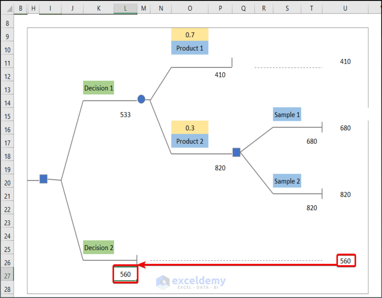
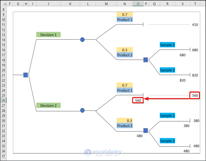
- Enter 560 in L27 (the value of U26).
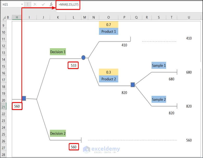
- Enter the following formula in H21.
=MAX(L15,L27)the MAX function returns the maximum value between L15 and L27.
The best decision in this dataset is 560.
Read More: How to Use Artificial Intelligence in Excel
Example 2 – Making a Decision Tree for 6 Events
Step 1: Create a Basic Outline of the Decision Tree
- Press CTRL+C & CTRL+V and recreate the figure.

Step 2: Label Decision Tree and Input Values
- Input the corresponding data and label the chart.

- Enter the following formula in O33.
=MAX(S31,S36)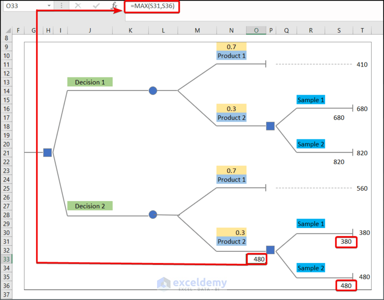
- Enter 560 into O26 to move the value in T25 into O26.
- Enter the following formula in O19.
=MAX(S17,S22)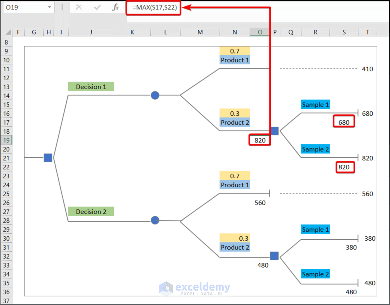
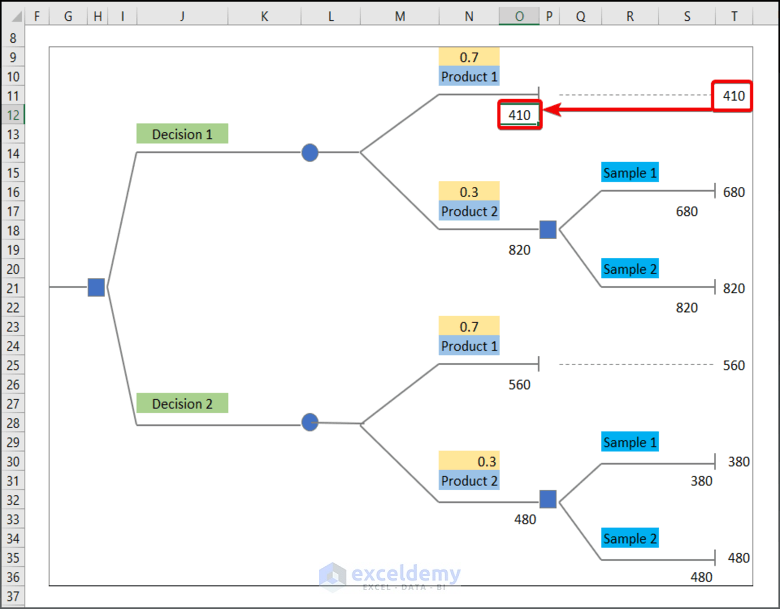
- Enter the data in T10 and 410 in O12.
- Enter the following formula in K15.
=IF(ABS(1-SUM(N9,N16))<=0.00001,SUM(N9 * O12,N16 * O19),NA())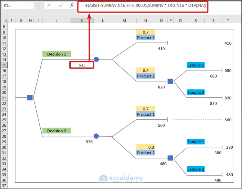
- Enter the following formula in K29.
=IF(ABS(1-SUM(N23,N30))<=0.00001,SUM(N23 * O26,N30 * O33),NA())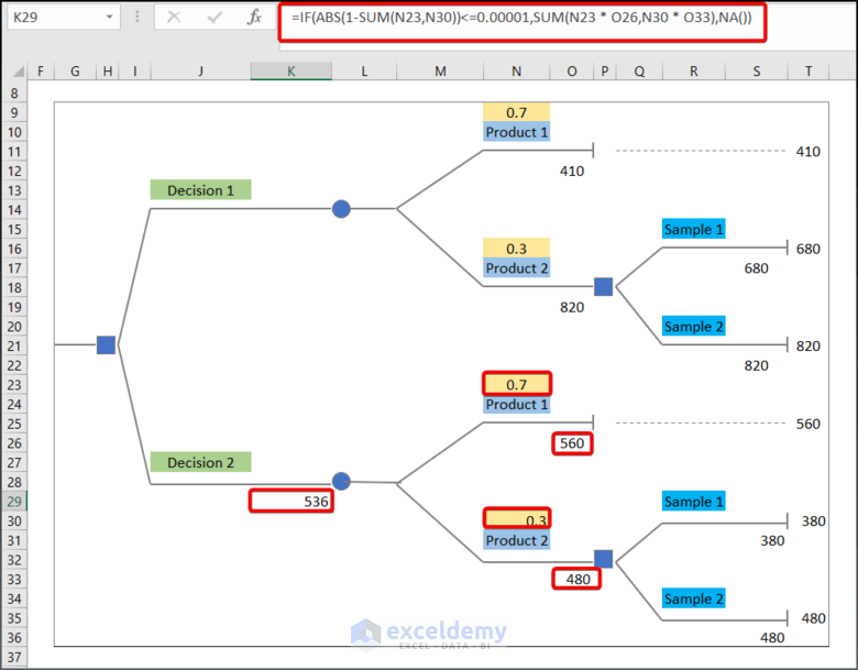
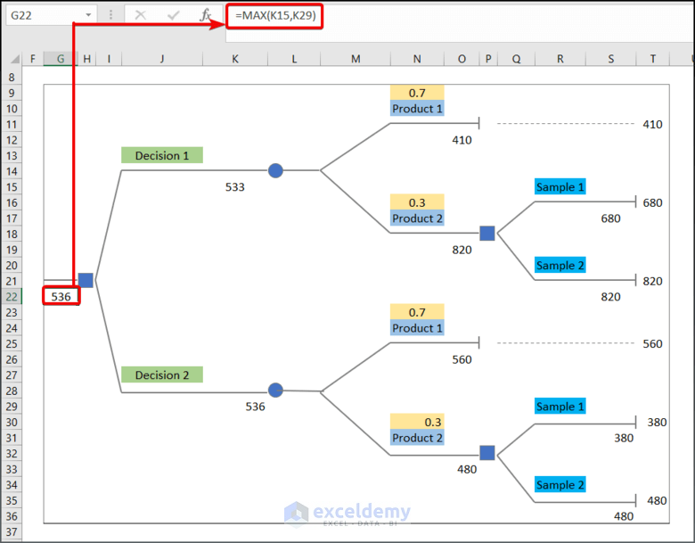
- Enter the following formula in G22 to find the maximum value of the two given decisions.
=MAX(K15,K29)This is the complete decision tree.
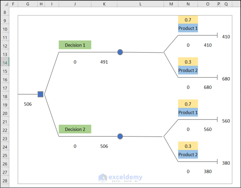
Example 3: Generating a Decision Tree with Equal Branches
- This is the dataset.
- Create two decision nodes and two chance nodes. This is the output.
Read More: How to Build Lottery Prediction Algorithm in Excel
Practice Section
Practice the decision tree algorithm in Excel.
Download Practice Workbook
Download and practice.
Related Articles
- How to Create Betting Algorithm in Excel
- How to Perform Machine Learning in Excel
- How to Use Fuzzy LOOKUP Algorithm in Excel
- How to Create Rainflow Counting Algorithm in Excel
<< Go Back to Algorithm in Excel | Learn Excel
Get FREE Advanced Excel Exercises with Solutions!- SUM(O9 * P12,O16 * P19) → The SUM function returns the product of O9*P12 and O16*P19.


I didn’t understand any things.
Hello Amit Kumar,
Thank you for your feedback. The article covers several examples step by step, but some parts can feel difficult if you are new to Decision Trees or machine learning in Excel. Please let us know which section was confusing, and we’ll try to explain it more clearly for you.
Regards,
ExcelDemy