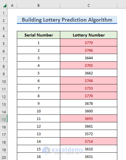
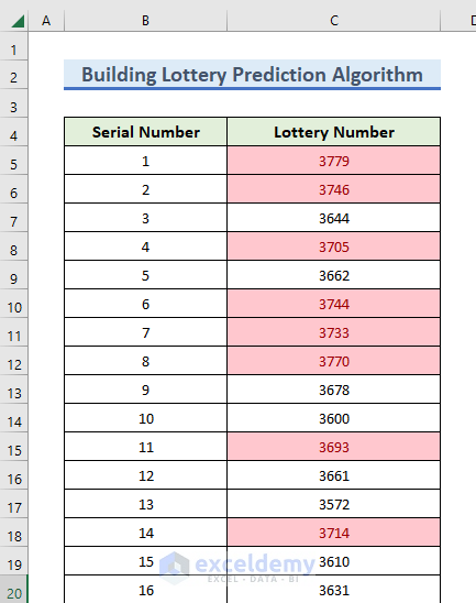
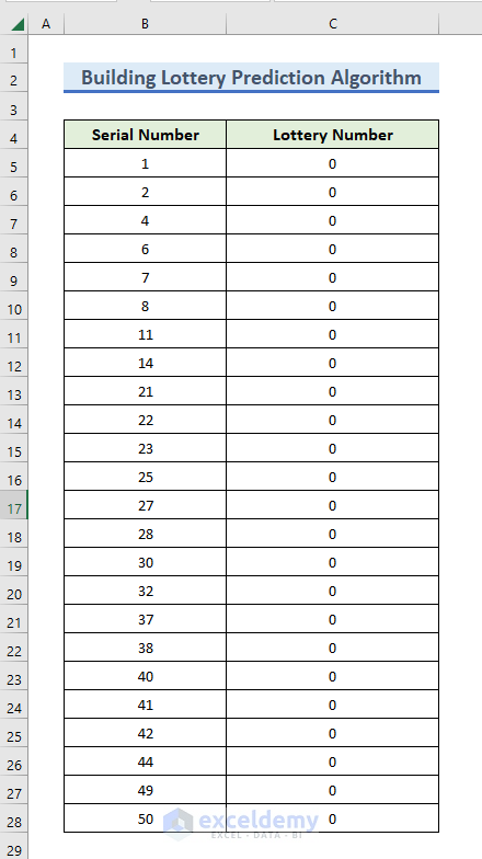
The sample dataset contains 2 columns. The 1st one with a series of lottery numbers and a 2nd column, in which the probability of selecting a serial number will be calculated.
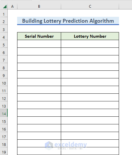
STEP 1: Create a Dataset
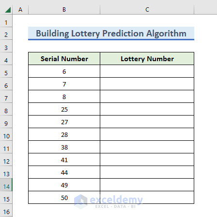
- Enter the serial number of the lottery in the Serial Number column (values can be manually inserted).
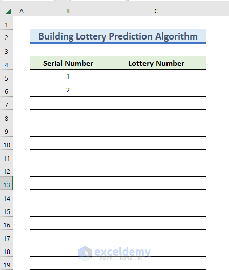
- To do it automatically, insert 1 and 2 in B5 and B6.
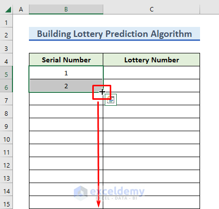
- Dag down the Fill Handle to fill the rest of the cells.
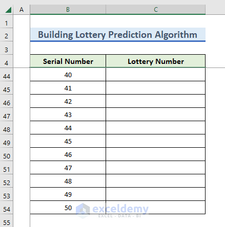
50 is the last serial number.
- Drag the Fill Handle down to B54.
The 50 serial numbers are inserted.
- Select the range.
STEP 2: Add Functions for Predictions
- Enter a formula to calculate the probability of a serial number.
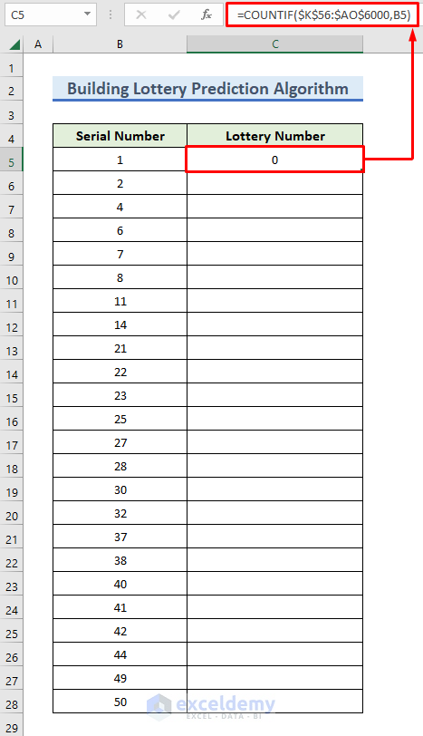
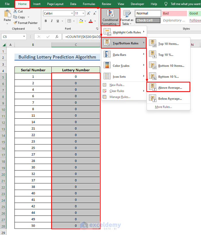
- Select C5 and enter the following formula using the COUNTIF function:
=COUNTIF($K$56:$AO$6000,B5)
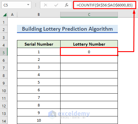
The formula counts the occurrence of serial number 1 in B5 in the range K56:AO6000.
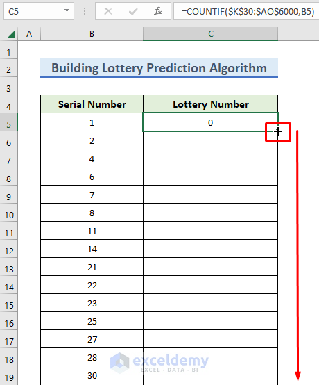
- Drag down the Fill Handle to fill all the cells.
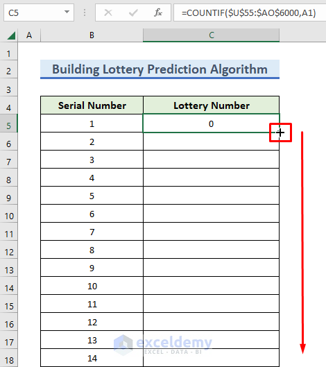
- All cells in column B are showing 0.
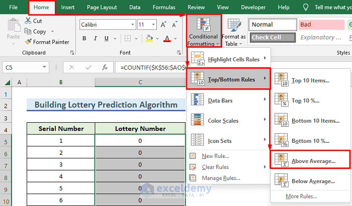
- Select column B.
- Go to the Home tab.
- In Styles, choose Conditional Formatting.
- Select Top/Button Rules >> Above Average.
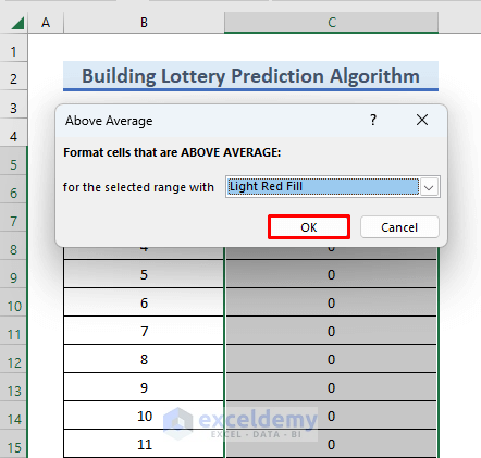
- In the dialog box will, select Light Red Fill from the drop-down menu.
Lottery numbers with a weightage above the average will show Light Red color.
- Click OK.
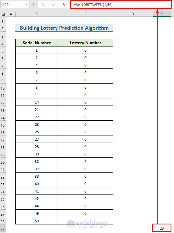
- Enter random numbers between 1 to 50.
- Select K55 and enter the following formula..
=RANDBETWEEN(1,50)
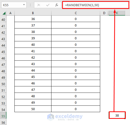
Here, the RANDBETWEEN function will insert any random integer number between 1 to 50.
- Press Ctrl + C, to copy K55 and drag the Fill handle to fill the other cells.
- Go to Name Box on the left side of the formula bar, where the cell number is shown.
- Enter the following formula to select the range:
K56:AO6000
This is the selected range.

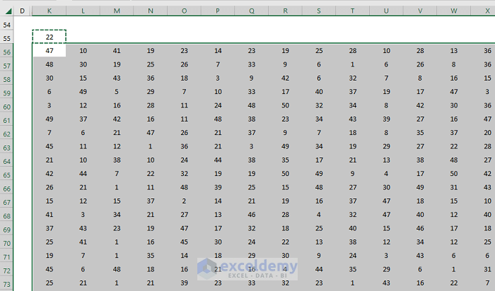
- Press Ctrl + V to paste the formula in the range.
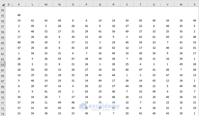
- Random numbers will be generated.
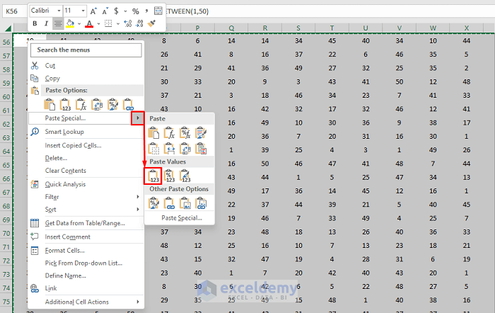
- Delete the formula in the range and replace it with values.
- Select K56:AO6000 and copy by pressing Ctrl + C. Values will change after every refresh.
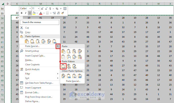
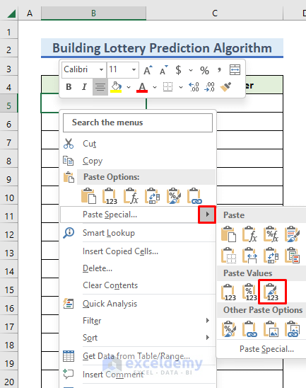
- Paste the range in the same range as the value format. Click K56 and right-click.
- In the dialog box, choose Paste Special.
- Select Paste Value.
The formula is replaced with generated random numbers.
Read More: How to Create Betting Algorithm in Excel
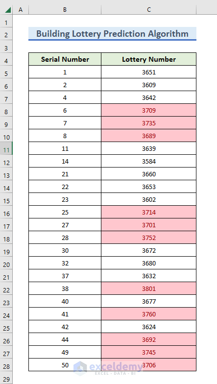
STEP 3: Predict the Most Frequent Numbers
- In column C, red cells indicate that the probability of selecting these red cells is greater than normal cells.
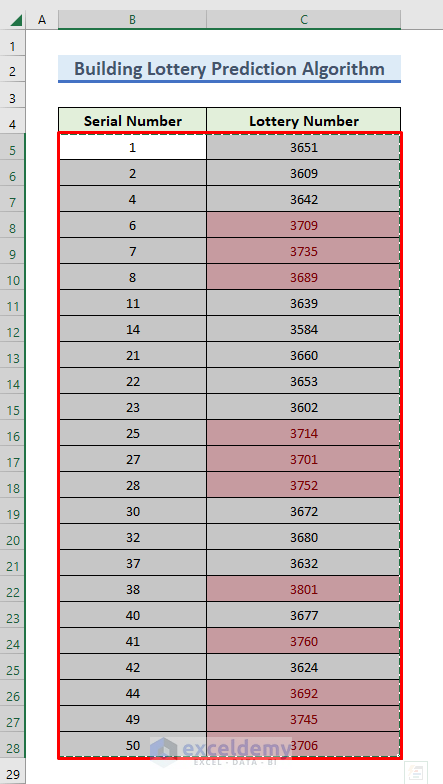
STEP 4: Repeating the Process by Using Highlighted Numbers
- Open a new worksheet.
- Copy the Serial Number and Lottery Number columns by pressing Ctrl + C.
- Paste these columns.
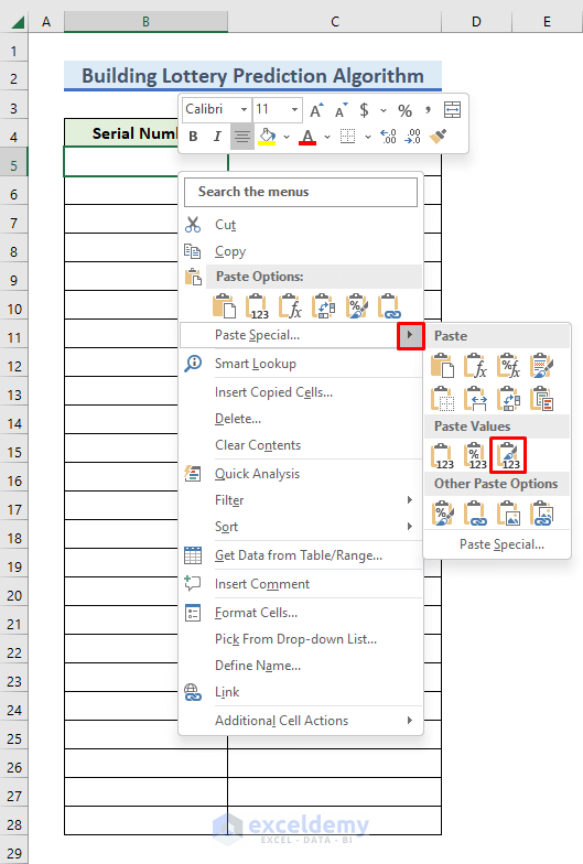
- Click B5 under the Serial Number header.
- Right-click and choose Paste Special.
- Select Values and Source Formatting to paste the cells and keep the same format.
This is the output.
The Serial Number column keeps the most probable serial numbers.
- Press Delete to delete the second column..
- Enter a formula to calculate the probability of the serial number.
- Select C5 and enter the following formula:
=COUNTIF($K$56:$AO$6000,B5)
- Drag down the Fill Handle to fill all cells with the formula.
Cells in column B are showing 0.
- Select column B.
- Go to the Home tab.
- In Styles, choose Conditional Formatting.
- Select Top/Button Rules >> Above Average.
- In the dialog box, select Light Red Fill from the drop-down menu.
- Click OK.
- To enter random numbers between 1 and 50: select K55 and enter the following formula.
=RANDBETWEEN(1,50)
- Press Enter to see the result.
- Copy K55 by pressing Ctrl + C.
- Go to Name box on the left side of the formula bar where the cell number is shown.
- Enter the following formula to select the range:
K56:AO6000
- Paste the formula by pressing Ctrl + V.
- Random numbers will be generated in this range.
- Delete the formula in the range and replace it with values.
- Select K56:AO6000 and copy by pressing Ctrl + C. Values will change after every refresh.
- Paste the range in the same range as the value format. Click K56 and right-click.
- In the dialog box, choose Paste Special.
- Select Paste Value.
The formula is replaced with generated random numbers
.
In column C., red cells indicate that the probability of selecting these red cells is greater than normal cells.
- Create 2 Excel sheets.
- Select columns B and C .
- Create a similar Excel worksheet.
- In this new worksheet, copy the Serial Number and Lottery Number by pressing Ctrl + C.
- Click B5 under the Serial Number header to paste these columns.
- Right-click and choose Paste Special.
- Select Values and Source Formatting to paste the cells and keep the same format.
In the Serial Number column, you have kept the most probable serial numbers.
- Delete the next column by pressing Delete.
- Follow the above procedure for the new Excel Sheet.
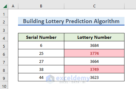
Final Output
After repeating the procedure twice, this will be the output.
Serial Numbers 25 and 38 are the most probable numbers.
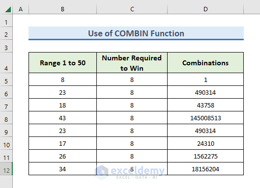
How to Determine Lottery Probability in Excel
STEPS:
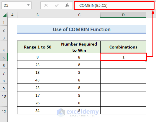
- Column B is our lottery ticket number.
- Column C is our output lucky lottery ticket number.
- To find the probability, select D5 and enter the following formula:
=COMBIN(B5:C5)
- Press Enter.
- The result is 0.
- Drag down the Fill Handle to fill all cells with the formula.
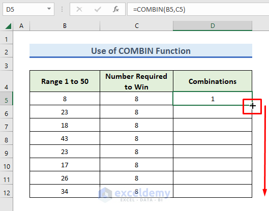
- The probability of the 23 serial number is 490314:1.
Download Practice Workbook
Download the following workbook.
Related Articles
- How to Use Fuzzy LOOKUP Algorithm in Excel
- How to Perform Machine Learning in Excel
- How to Use Artificial Intelligence in Excel
- How to Make Decision Tree Algorithm in Excel
- How to Create Rainflow Counting Algorithm in Excel
<< Go Back to Algorithm in Excel | Learn Excel
Get FREE Advanced Excel Exercises with Solutions!

U must be kidding! This is not “the way” how to do it no where. It’s pure luck if u target at least 1 number right out of million try’s. U should convert your data set to [0,1] or [-1,1] in time series manor 8u can also use machine learning or xlstat), then do serious analysis on it to discover variance and clusters and for each cluster do separate time series forecast with fine tuning (tuning from cluster to cluster will be much different, u basically seek for average in each row in cluster to achieve high confidence as u wont hit proper number ever time in every cell). Then u evaluate each row in cluster for accuracy in that cluster for each prediction to see if confidence gets up and down against known values for particular time data column. If u do time series forecast even with fine tuning on entire dataset at once u get average 40 to 60% of accuracy and result will jump a lot for each prediction. That isn’t near enough to make valid choice and u just might get 1 or at best 2 number right in best case (data pattern and variance). That’s why no one cracked Lotto yet ! And for machine learning u need a lot of data. How do u get a lot of data out of little data, well that is another pair of socks. So your proposed solution is nothing but at least function exercise for excel user at very basic level.
Hello Jeff,
Thanks for your insightful feedback! You’re absolutely right that lottery predictions are mostly based on luck, and the approach in the article is more of an introductory exercise using Excel. For accurate forecasting, more advanced methods, such as machine learning and time series analysis, are necessary. While this article serves as a basic guide for Excel enthusiasts, we appreciate your perspective and will consider updating it with a clearer disclaimer about the limitations of such predictions.
Regards
ExcelDemy