How to Use Fuzzy LOOKUP Algorithm in Excel: 2 Easy Methods

Method 1 – Matching Obtained Marks by Fuzzy LOOKUP Algorithm

Steps:

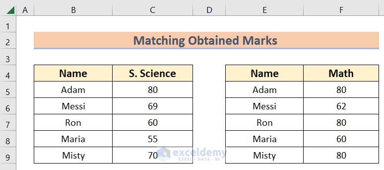
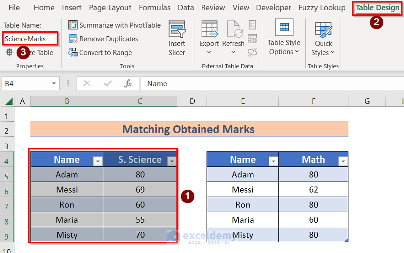
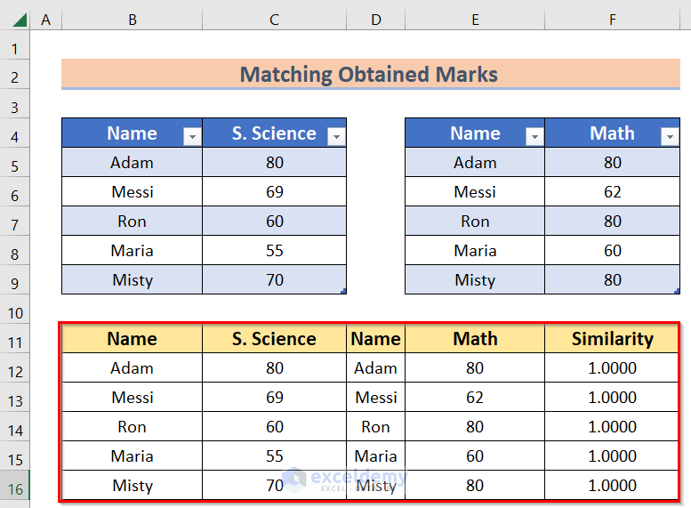
• In the first table, Name in column B and Science in Column C. In the second table, Name in column E and Math in Column F. We will use this dataset to explain the whole method.

• If you don’t have Fuzzy LOOKUP built-in in Excel, you have to download it from Microsoft Excel Note that we are using Microsoft 365 in this article.

• You have to install the downloaded file. If you restart the Excel file again, you will see the Fuzzy LOOKUP Add-in in the Excel tab.

• Select the first data table and press the Ctrl+L to convert the data range into a data table.

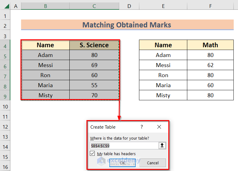
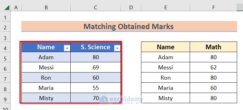
• Get the first data table accordingly.

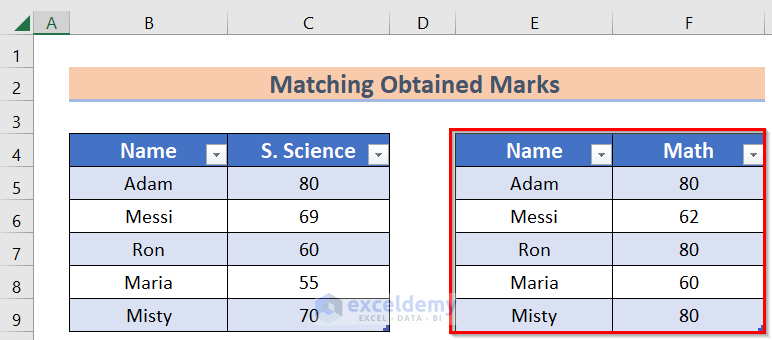
• Repeat the same process to get the second data table similar to the below image.

• Click the table and go to the Table Design tab, and in the Table Name option set the name of the table accordingly. We set the table’s name as ScienceMarks.

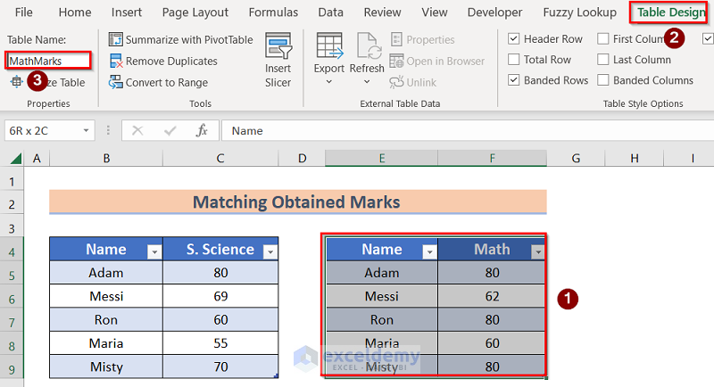
• If you want to select a different name for the table, you have to select the second table and go to the Table Design tab, and the Table Name option sets the name of the table. We set the name of the table as MathMarks. Note that you have to name the table again individually.

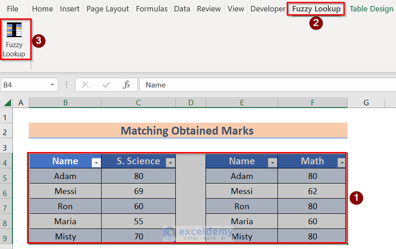
• Select the two tables and click on the Fuzzy Lookup feature.

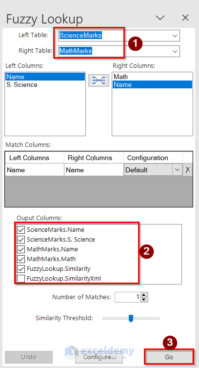
• In the Fuzzy Lookup feature, select the Left Table and Right Table accordingly. We set the ScienceMarks table as the Left table and the MathMarks table as the Right table.

• Tick the cells in the output columns option and press GO.

• Get a new table where you will find similarities between the two tables on the same worksheet.

We learned how to use the fuzzy LOOKUP algorithm by using the Fuzzy LOOKUP Add-in feature.

Method 2 – Merging Official Data by Fuzzy LOOKUP Algorithm

Steps:

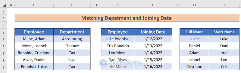
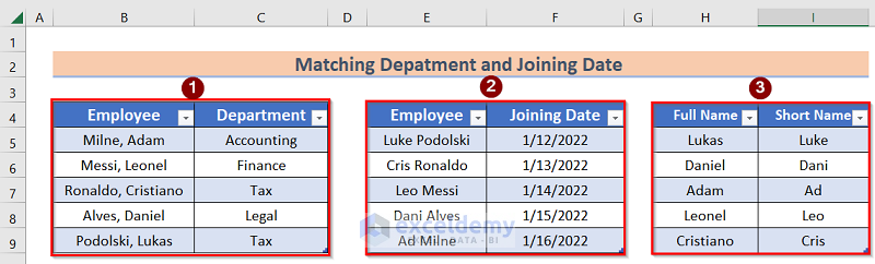
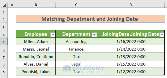
• We have three data tables. The first table consists of Employee and Department, in the second table, Employee and Joining Date and in the third table, Full Names and Short Names. We will use this dataset to explain the whole process.

• Convert the data ranges into tables by following the steps of the first method.

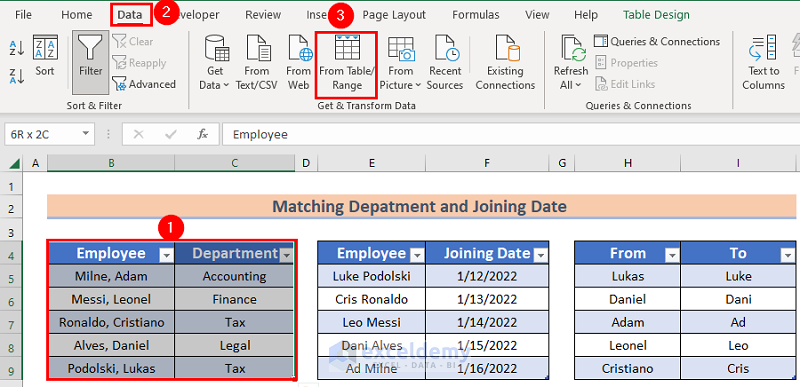
• Select the first data table >> Data >> From Table/Range. You have to change the headings of one table to From and To. We changed the headings of the last table headings to From and To.

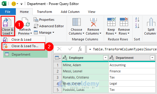
• In the Power Query Editor, you will get the result, and then in the Close and Load option, select the Close and Load to option.

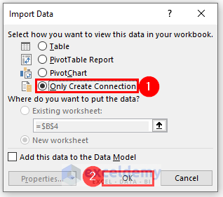
• The Import Data window will open on the screen. In this window, select the Only Create Connection option and press OK.

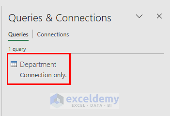
• You will find the new Queries on the right side of the window.

• Repeat the same process to connect all the tables in this section.

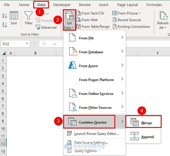
• Go to Data >> Get Data >> Combine Queries >> Merge options.

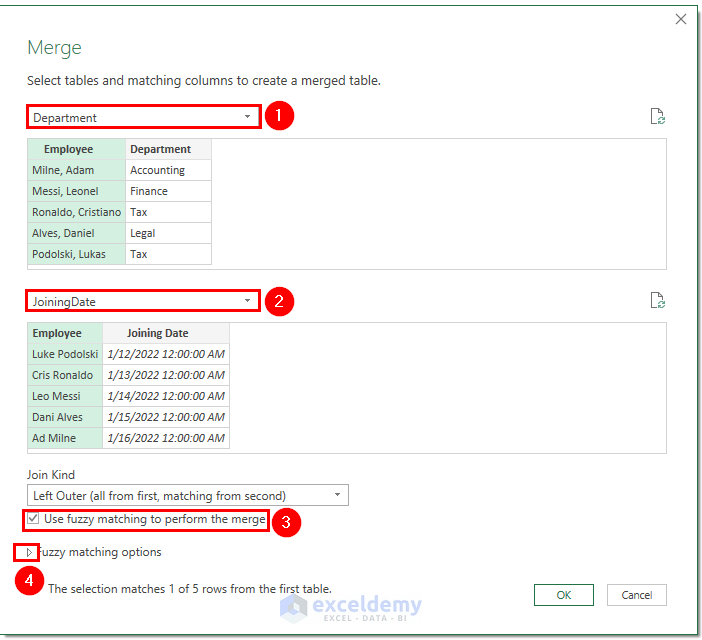
• In the Merge window, select the first two tables. Select the first column of the table manually in the section. Click Use fuzzy matching to perform option and click on the triangle named Fuzzy matching feature.

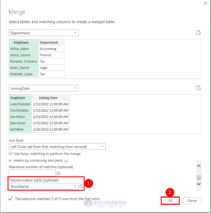
• In the Fuzzy matching options, select the third table in the Transformation Table option and press OK.

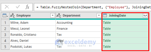
• Get the result, but the Joining Date column is empty initially.

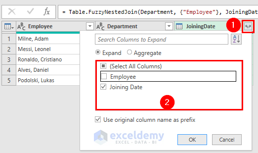
• Click on the arrow sign and select only the Joining Date option. Press OK.

• Get the result in the Merge1 section, and press Close and Load to get the result.

• Get the final result accordingly.

You learned how to use the fuzzy LOOKUP algorithm using the fuzzy match ( Power Query) in Excel.

Download Practice Workbook

You can download the practice workbook from here.

Related Articles

• How to Build Lottery Prediction Algorithm in Excel
• How to Create Betting Algorithm in Excel
• How to Perform Machine Learning in Excel
• How to Use Artificial Intelligence in Excel
• How to Make Decision Tree Algorithm in Excel
• How to Create Rainflow Counting Algorithm in Excel

<< Go Back to Algorithm in Excel | Learn Excel