How to Use Artificial Intelligence in Excel (4 Easy Examples)

Example 1 – Evaluating Intelligence Suggestions with Analysis

When you are working with a large dataset and want to insert a chart, the Analyze Data option has made it easier. It automatically gives you some suggestions.

Steps:

• Select the entire data range and move to the Analyze Data from the Analysis section.

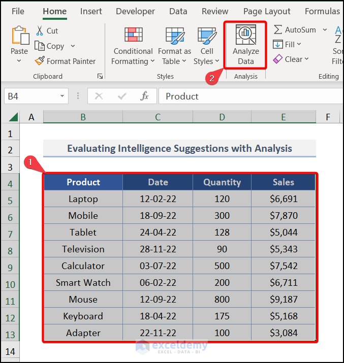
• The Analyze Data panel appears. You can choose different charts according to your preference. It also shows some intelligent suggestions for choosing your decision towards your company or product-related information.

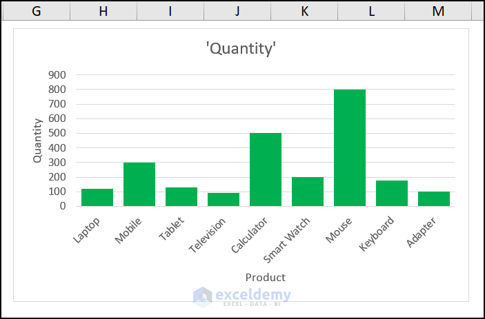
• You can insert any of the charts at your preference that is relevant to your dataset. We have inserted a chart for better visualization.

Read More: How to Make a Decision Tree Algorithm in Excel

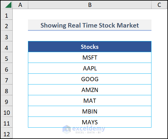
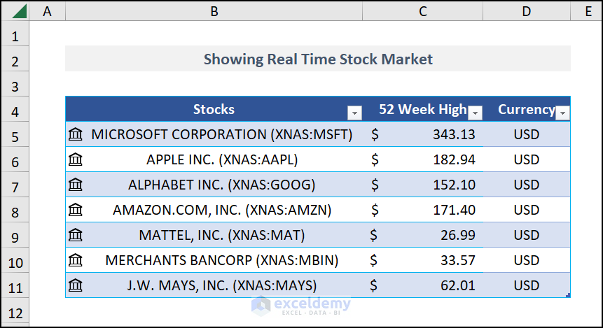
Example 2 – Showing Real-Time Stock Prices

Steps:

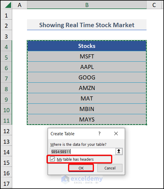
• Write down some stock’s short codes like the image below:

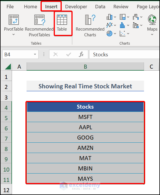
• Select the entire data range.
• Go to the Insert tab.
• Choose Table from the Tables group.

• The Create Table window appears. Check the My table has headers box and hit OK.

• Select the range of the data table and hover over the Data tab.
• Pick Stocks from the Data Types section.

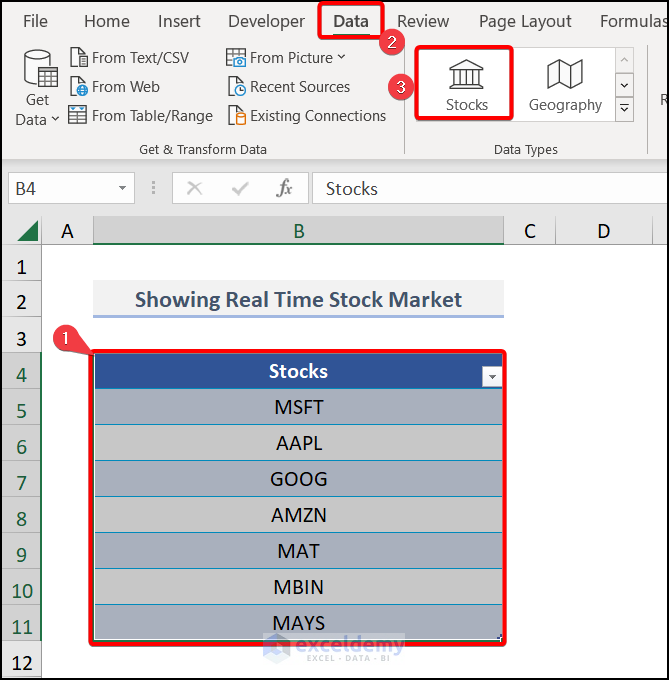
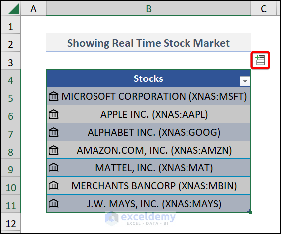
• The short code will turn into the stock names.
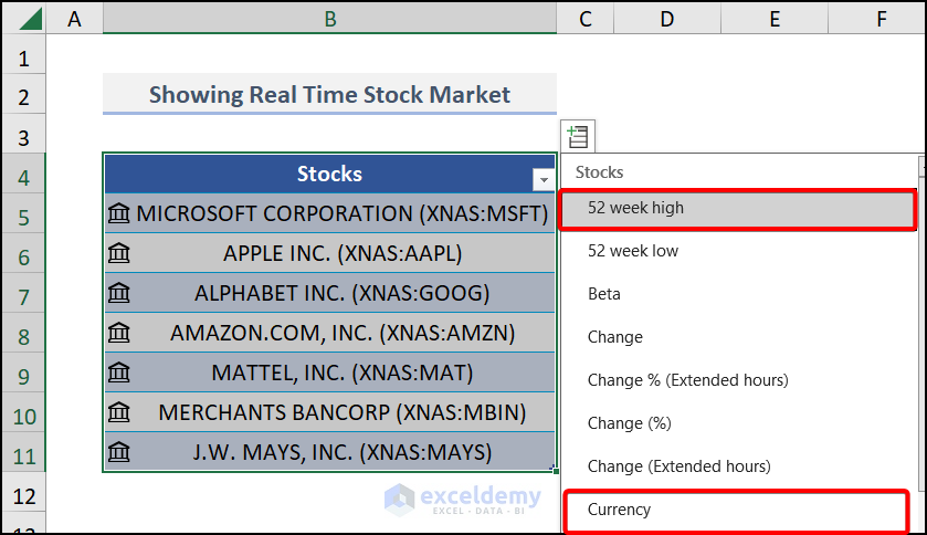
• You can add a column from the Add Column command which is in the right top corner of your data table.

• We chose 52 weeks high and Currency from the column section. There are a lot of options available in the Add Column section.

• You can see the column has been added to your stock section.

• You can click on the stock sign and get important information about the related stocks.

Read More: How to Perform Machine Learning in Excel

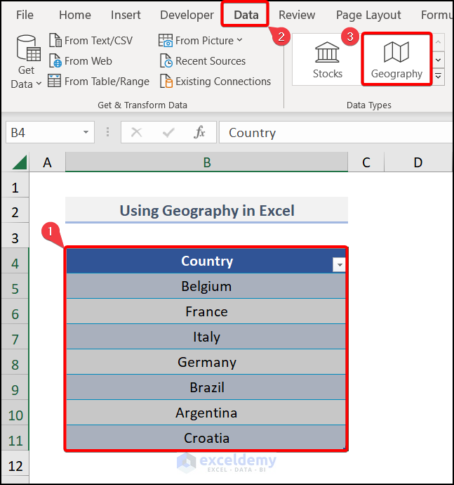
Example 3 – Using Geography in Excel

Steps:

• Write country or region names and make a table with the data as mentioned before.
• Navigate to the Data tab and pick Geography from the Data Types group.

• Add columns from the Add Column section from the upper right corner of the data table.

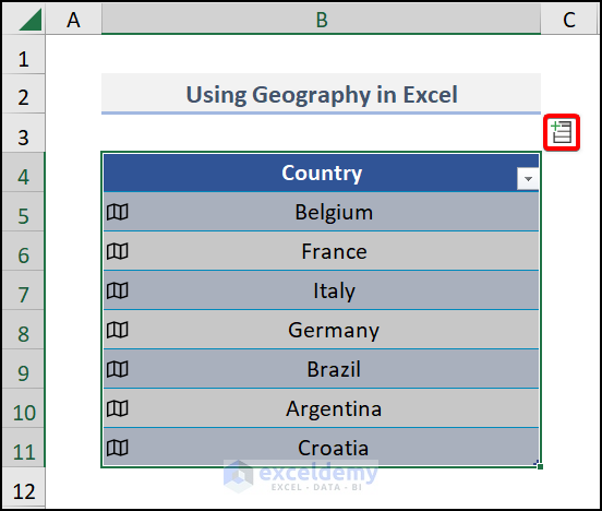
• Pick some columns to your preference.

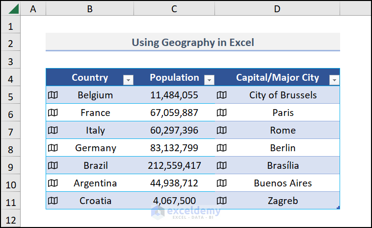
If you click on the geographic sign, you can find the available information on the internet about that specific region.

Example 4 – Employing Dynamic Array Functions

Steps:

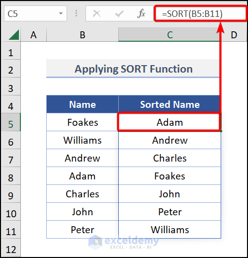
• Go to cell C5 and insert the formula:

This function will sort the data of B5:B11 alphabetically as you can see in the image.

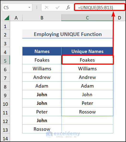
• If you have duplicates in your dataset then you can use the UNIQUE function to remove the duplicates:

The above syntax will remove the duplicate values from the range of B5:B13.

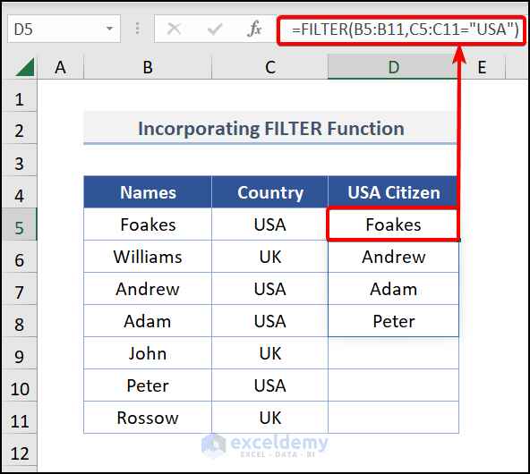
If you want to choose specific data based on your criteria. In the below dataset, you want to filter the data to know the USA citizen.

• Go to cell D5 and insert this formula:

The function will filter the data in the B5:B11 in the criteria_range C5:C11 for the criteria of USA.

You can also use SORTBY and SEQUENCE functions.

Practice Section

We have provided a practice section on each sheet on the right side for your practice. Please do it by yourself.

Download Practice Workbook

Download the following practice workbook. It will help you to realize the topic more clearly.

Related Articles

• How to Build Lottery Prediction Algorithm in Excel
• How to Create Betting Algorithm in Excel
• How to Use Fuzzy LOOKUP Algorithm in Excel
• How to Create Rainflow Counting Algorithm in Excel

<< Go Back to Algorithm in Excel | Learn Excel