In this article, we will discuss the calculation process of Double Declining Depreciation in Excel. The Double Declining Depreciation is one of the accelerated methods of calculating depreciation. Here, the depreciation percentage is a multiple of the straight-line depreciation. We often need this method to calculate the depreciation of an asset. This results in good estimations for assets with a long-life span. In this instance, we will calculate the Double Declining Depreciation in 2 ways.
How to Calculate Double Declining Depreciation in Excel: 2 Ways
In this article, we will calculate the Double Declining Depreciation in 2 ways. Firstly, we will use the formula for the method manually in Excel to calculate the depreciation. Then, we will use the DDB function to do the task.
1. Using Arithmetic Formula
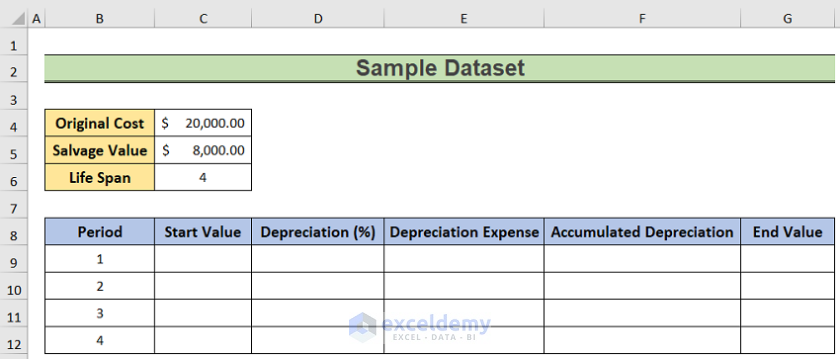
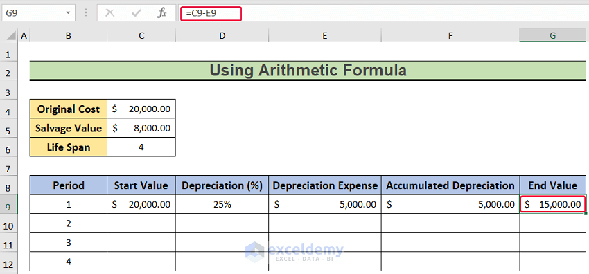
In this method, we will calculate the double declining depreciation in Excel manually. Here, we have an asset which has an original cost of $20000 and a salvage value of $8000 with a life span of 4 years. We will calculate its depreciation using the Double Declining Depreciation method.
Steps:
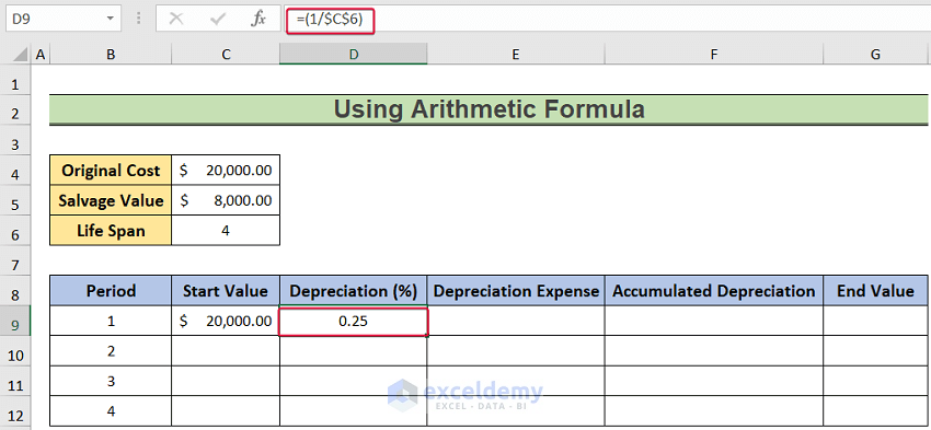
- Firstly, select the D9 cell and type,
=1/$C$6- Secondly, hit Enter.
- Consequently, we will get the Depreciation Percentage for period one.
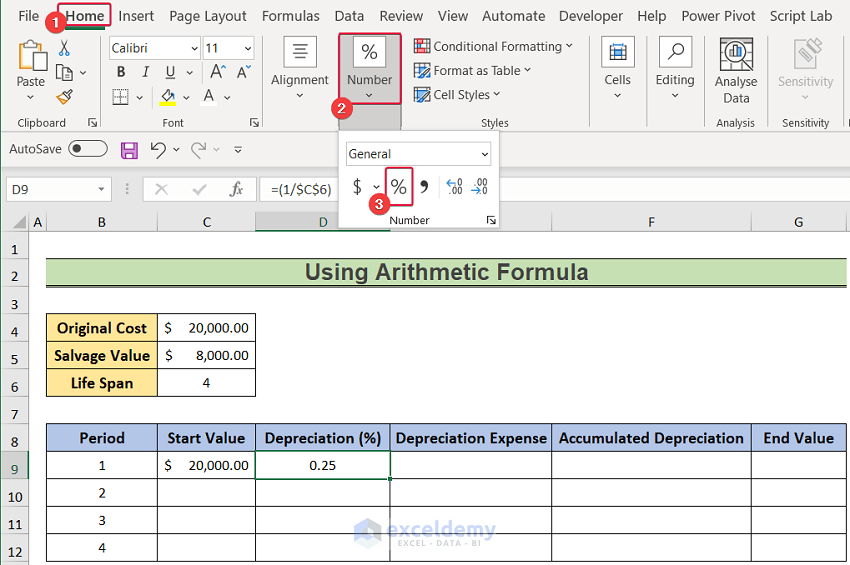
- Thirdly, go to the Number group in the Home tab and make the number a percentage.
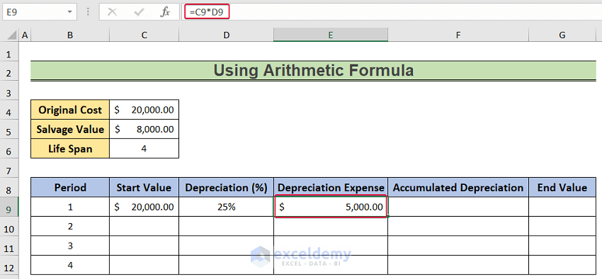
- Then, click on the E9 cell and enter,
=C9*D9- Hit Enter after that.
- As a result, we will get the Depreciation Percentage for the asset.
- Then, select the F9 cell and write,
=E9- Press Enter.

- Finally, choose the G9 cell and enter the following formula,
=C9-E9- Then, press Enter.
- As a result, we will get the End Value for the first year.
- After that, click on the C10 cell and enter the following,
=G9- Hit the Enter button afterwards.

- Next, choose the E10 cell and type the following formula in the cell,
=C10*D10- As a result, we will get the Depreciation Expense for year two.

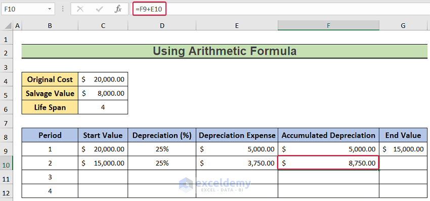
- Thereafter, click on the F10 cell and type,
=F9+E10- Consequently, we will get the accumulated depreciation for the first two years.
- Again, select the G10 cell and enter,
=C10-E10- As a result, we will get the End Value for the year 2.

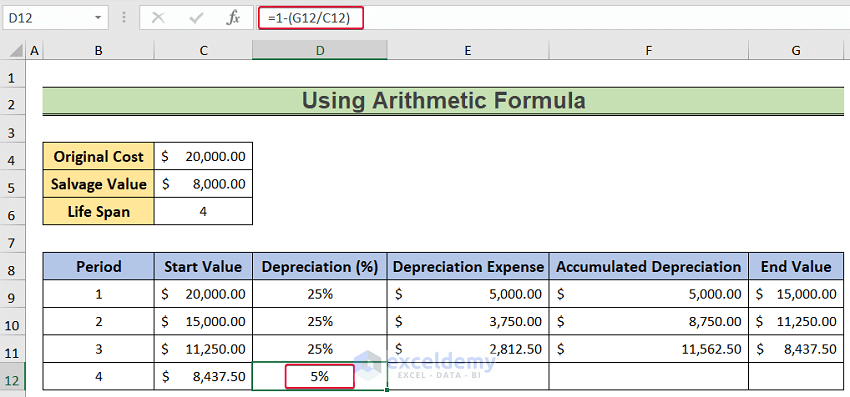
- Repeat the same process for the next upcoming years unless the End Value becomes less than or equal to the salvage value.

- In this case, the end value becomes less than $8000 at year 4.
- Here, we will change the Depreciation Percentage
- So, choose the D12 cell and write the following,
=1-(G12/C12)- Then, hit Enter.
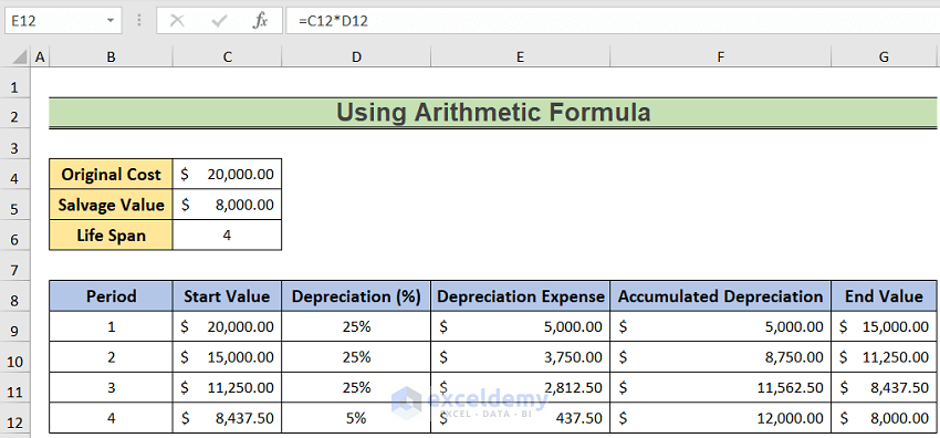
- Now, repeat the same calculations for the Depreciation Expense, Accumulated Depreciation and End Value.
- Finally, we will get the salvage value for the asset after 4 years.
Read More: How to Calculate Accumulated Depreciation in Excel
2. Applying DDB Function
The DDB function is the dedicated function to calculate depreciation of an asset using the Double Declining Depreciation method in Excel. The function takes cost, salvage value, life span and period of depreciation as arguments. In this method, we will utilize this function to do the calculation.
Steps:
- To begin with, select the D9 cell and enter,
=DDB($C$4,$C$5,$C$6,B9)- Then, press Enter.
- As a result, we will get the Depreciation Expense for the asset for year one.

- After that, choose the E9 cell and write the following formula,
=C9-D9- Hit Enter.
- This will result in the End Value for year one.

- Next, choose the C10 cell and enter,
=E9- Press Enter after that.

- Thereafter, choose the D10 cell and type,
=DDB($C$4,$C$5,$C$6,B10)- Then, hit Enter.
- Consequently, we will have the Depreciation Expense for the year two.

- Afterward, click on the E10 cell and write the following formula,
=C10-D10- Press Enter.

- Repeat the process for the next 2 years.

- Finally, select the D13 cell and enter the formula below,
=SUM(D9:D12)- Press the Enter button after that.
- As a result, we will get the Total Depreciation for the asset using the double depreciation method by applying the SUM function.

Read More: How to Apply Declining Balance Depreciation Formula in Excel
Download Practice Workbook
You can download the practice workbook here.
Conclusion
In this article, we have talked about calculating Double Declining Depreciation in Excel in two ways. These methods will allow users to calculate the depreciation of their assets using the double depreciation method easily in Excel. If you have any questions regarding this essay, feel free to let us know in the comments.
Related Articles
- How to Calculate Straight Line Depreciation Using Formula in Excel
- How to Use WDV Method of Depreciation Formula in Excel
- Calculate Sum of Years Digits Depreciation with Formula in Excel
- Units of Production Depreciation Method with Formula in Excel
- How to Use SLM Method of Depreciation Formula in Excel
- How to Use MACRS Depreciation Formula in Excel
- How to Use Formula to Calculate Car Depreciation in Excel
<< Go Back to Depreciation Formula In Excel|Excel Formulas for Finance|Excel for Finance|Learn Excel
Get FREE Advanced Excel Exercises with Solutions!
