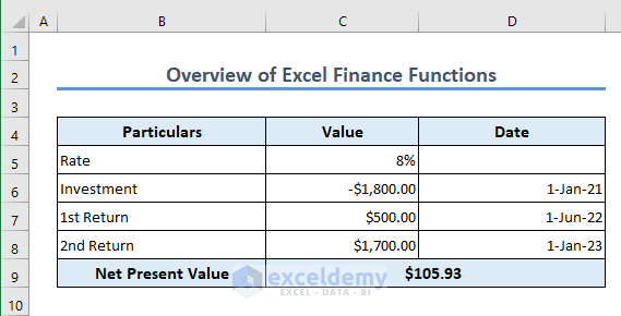
Excel Formulas for Finance: An Easy Guide

In this article, we will learn 18 frequently used Excel formulas for finance that cover a wide range of financial calculations, allowing you to make more informed decisions. The formulas are based on FV, FVSCHEDULE, PV, NPV, XNPV, IRR, MIRR, XIRR, NPER, PMT, IPMT, PPMT, RATE, EFFECT, NOMINAL, SLN, DB, and SLOPE functions.

From determining the future value of an investment using the FV function to analyze the net present value with the NPV function, these Excel formulas for finance help financial professionals, analysts, and even individual investors.

Whether you’re working on financial forecasting, evaluating investment opportunities, or managing your personal finances, understanding these formulas will help you a lot.

This easy-to-follow guide will provide a concise overview of each formula, explaining its purpose and how to use it effectively. By the end of this article, you’ll have a solid foundation in using Excel for financial analysis.

Overview of Excel Formulas for Finance

Download Practice Workbook

Excel Formula for Finance.xlsx

Formula 1 – FV Function

The FV function calculates the future value of an investment or loan based on a series of periodic payments and a fixed interest rate.

Suppose you have taken a loan of $200 at a semi-annual rate of 8%. This means the loan is repaid twice a year. The annual interest rate would be 16%.

The loan term is 3 years. We can now calculate the future value of this $200 using the following formula in cell C9.

=FV(C5,C8,C6,-C7)

In the formula, we have a minus (–) sign before C7, because the loan repayment is a cash outflow.

Formula 2 – FVSCHEDULE Function

In the previous example, we have considered a constant periodic interest rate. But this may not always be the case. Your periodic interest rate may vary over time. In such cases, if you want to get the future value of a certain amount, you can use the FVSCHEDULE function.

In the following example, we have taken 3 different periodic interest rates. The repayment is annual here. The formula in C11 is,

=FVSCHEDULE(C5,C8:C10)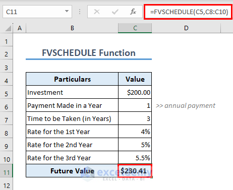

Formula 3 – PV Function

Excel also offers you the option to calculate the present value of a certain future value. The function to be used in such cases is the PV function. The formula in C9 is,

=PV(C5,C8,C6,-C7)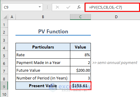

Formula 4 – NPV Function

NPV stands for Net Present Value. As the name suggests, NPV will get you the net present value of a series of cash flows.

Let’s assume that you have invested $1800 in a project. The return in the 1st year will be $500 and $1700 in the 2nd year.

To understand whether the project is profitable, you can use the NPV function. A positive NPV value will indicate that the project is profitable. The formula in C9 is

=-C6+NPV(C5,C7:C8)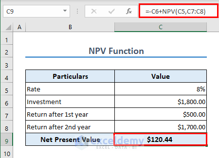

Note:

The initial investment is a cash outflow. That’s why a minus (–) sign has been used before C6.
The initial investment is not inside the NPV function. Because the initial investment is made at present. The returns are to be received in the future, that’s why they are inside the NPV function.
By default, the first value inside the NPV function (in our case it is C7) is the cash flow after the 1st year, the second value inside the NPV function (in our case it is C8) is the cash flow after the 2nd year, and so on.

Formula 5 – XNPV Function

An advanced version of the previous NPV function is the XNPV function. In this function, you can input the date of the cash flows and Excel will get you the net present value. The formula to calculate XNPV in the following is,

=XNPV(C5,C6:C8,D6:D8)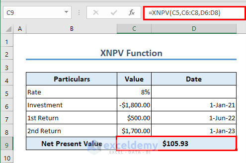

Formula 6 – IRR Function

IRR stands for Internal Rate of Return. It is a financial metric used to evaluate the potential profitability of an investment or project. The Internal Rate of Return represents the discount rate at which the net present value (NPV) of the investment becomes zero.

In simpler terms, the IRR is the rate at which an investment breaks even. It is the interest rate that makes the present value of the investment’s cash inflows equal to the present value of its cash outflows.

You can calculate the IRR using the IRR function if you have the cash flows over time. The formula in C9 is,

=IRR(C6:C8)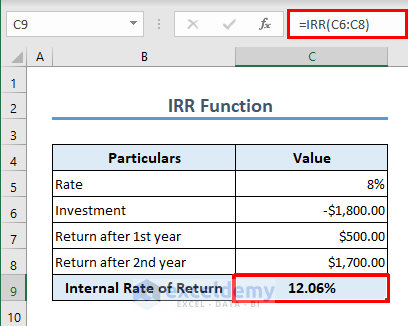

Formula 7 – MIRR Function

MIRR (Modified Internal Rate of Return) considers the reinvestment of the net present value of the capital inflows at a rate equal to the firm’s cost of capital.

It gives a more realistic estimation of the profitability of an investment compared to the internal rate of return. The MIRR function considers both the finance and reinvest rates to calculate the modified internal rate of return. The formula in C10 is

=MIRR(C5:C7,C8,C9)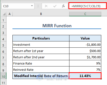

Formula 8 – XIRR Function

If you want to specify the dates of the cash flows, you can use the XIRR function.

The formula in C9 is

=XIRR(C6:C8,D6:D8)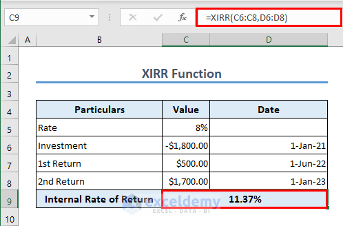

Formula 9 – NPER Function

The NPER function is used to calculate the payment period of any loan at a specific rate. We have calculated the number of periods using the following formula in cell C8.

=NPER(C5,C6,-C7)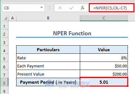

The payment period is approximately 5 years. Remember that these payments include both the principal and interest amount.

Formula 10 – PMT Function

To calculate each payment against a loan, you can use the PMT function. The formula in cell C9 is

=PMT(C5,C8,-C7)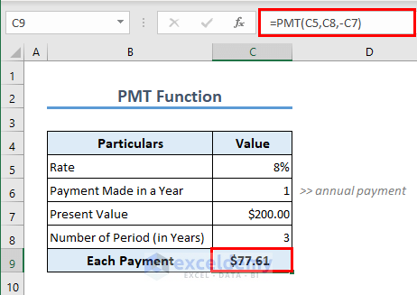

Formula 11 – IPMT Function

When you pay a loan, you pay both the principal and the interest. So each payment you make has 2 portions, one for the interest and another for the principal. You can get the portion for the interest using the IPMT function. To get the interest portion in your first payment after 1 year, the formula is

=IPMT(C5,1,C8,-C7)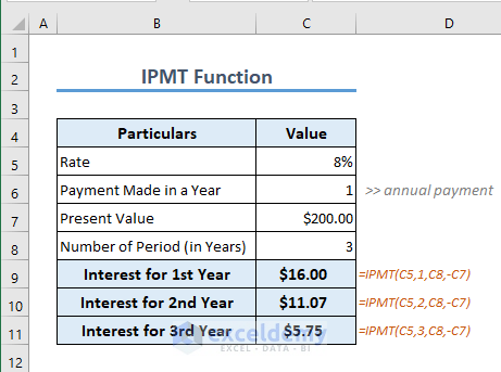

Follow the same process to get the interest portion for the rest of the payments.

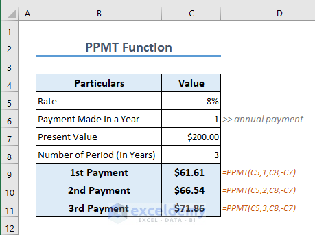
Formula 12 – PPMT Function

If you want to get the principal portion of any of the payments, you can use the PPMT function.

The formula to calculate the principal portion for the 1st payment is

=PPMT(C5,1,C8,-C7)

Follow the same process to get the principal portion of your subsequent payments.

Formula 13 – RATE Function

If you want to calculate the periodic interest rate of any loan, you can use the RATE function. The formula in cell C8 is

=RATE(C5,C6,-C7)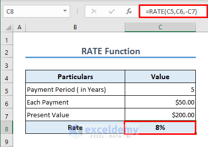

Formula 14 – EFFECT Function

The effective interest rate is the actual interest rate you earn or pay on a loan or investment when you consider how often the loan is compounded. It includes both the original amount of money and any interest you’ve already earned or paid.

It helps you understand the real cost or return of your money over time. It’s different from the advertised interest rate, which doesn’t take into account how often the interest is added to your account.

You can use the EFFECT function to get the effective interest rate. The formula in C7 is

=EFFECT(C5,C6)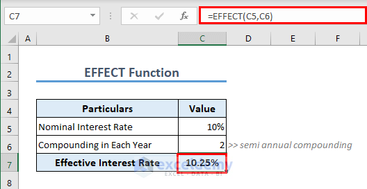

Formula 15 – NOMINAL Function

To get the nominal interest rate from the effective interest rate, you can use the NOMINAL function. The formula in C7 is

=NOMINAL(C5,C6)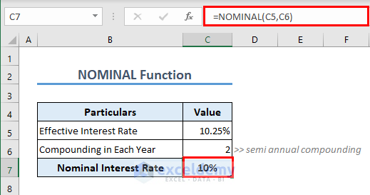

Formula 16 – SLN Function

Depreciation is an important concept in finance. There are different ways to calculate the depreciation for an asset. One of the simplest ones is the Straight Line Method. In this method, we assume that the asset depreciates linearly.

Excel offers the SLN function to measure the depreciation of an asset. Let’s assume the cost of an asset is $10000. The life cycle is 7 years with a salvage value of $100.

The formula in C8 is

=SLN(C5,C7,C6)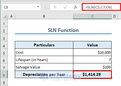

Formula 17 – DB Function

The straight-line method is not a very practical approach to calculate the depreciation of an asset. A better option is to calculate it using the Double Declining Balance Method. It is an accelerated depreciation method, meaning it assigns a higher depreciation expense in the earlier years of the asset’s life and gradually reduces it over time.

The DB function is frequently used to measure depreciation in such cases. The formula for the depreciation in the 1st year is in cell C8.

=DB(C5,C7,C6,1)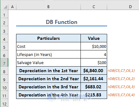

Formula 18 – SLOPE Function

We can correlate 2 variables in Excel using the SLOPE function. In the dataset, we have 2 variables, Advertising Expense, and Sales Revenue. We will try to find out how advertising expenses (independent variable) are affecting sales revenue (dependent variable). The formula in cell D11 is

=SLOPE(D5:D9,C5:C9)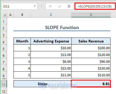

The result indicates that there is a positive correlation, and for a change in 1 unit of advertising expense, there is an 8.81 unit change in sales revenue.

Things to Remember

Cash outflows are negative and inflows are positive.
Effective interest rates consider compounding factors.
Slopes illustrate relationships between variables.

Frequently Asked Questions

1. How is the IRR different from the ROI?

The IRR calculates the rate of return based on the timing and magnitude of cash flows, while the return on investment (ROI) measures the profitability of an investment by comparing the net profit to the initial investment.

2. What is the significance of IRR?

The significance of IRR is:

If IRR > Required Rate of Return: The project is potentially profitable and meets the desired return expectations.
If IRR = Required Rate of Return: The project meets the minimum financial criteria but may not provide excess returns.
If IRR < Required Rate of Return: The project may not be financially viable or attractive based on desired profitability standards.

3. Can I combine the DB or SLN function with other Excel functions?

Yes, you can combine the DB or SLN function with other Excel functions to perform more complex calculations or build depreciation schedules.

Excel Formulas for Finance: Knowledge Hub

<< Go Back to Excel for Finance | Learn Excel

Get FREE Advanced Excel Exercises with Solutions!