In Microsoft Excel, the MIRR function estimates the likely profitability of an investment or project.
Introduction to the MIRR Function
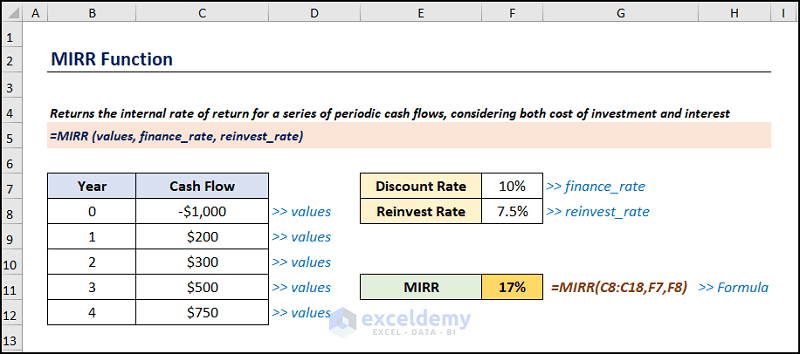
MIRR (Modified Internal Rate of Return) considers the reinvestment of the net present value (calculated with the NPV function) of the capital inflows at a rate equal to the firm’s cost of capital.
MIRR gives a more realistic estimation of the profitability of an investment compared to the internal rate of return.
- Function Objective:
The MIRR function considers both the finance and reinvest rates to calculate the modified internal rate of return.
- Syntax:
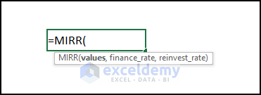
=MIRR(values, finance_rate, reinvest_rate)
- Argument Explanation:
| Argument | Required/Optional | Explanation |
|---|---|---|
| values | Required | An array consisting of the yearly cash flows |
| finance_rate | Required | The discount rate as a percentage |
| reinvest_rate | Required | The rate of interest (as a percentage) on the reinvested yearly cash flows |
- Return Parameter:
The Modified Internal Rate of Return while taking into account the discount rate and reinvestment rate.
How to Use the MIRR Function in Excel: 3 Examples
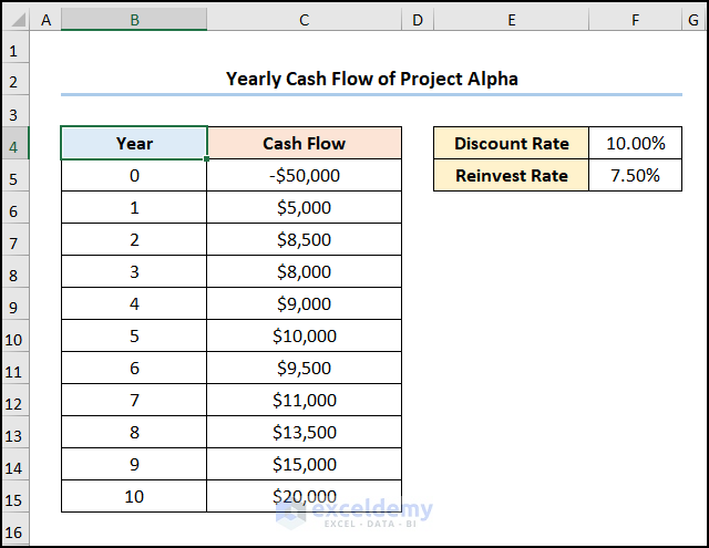
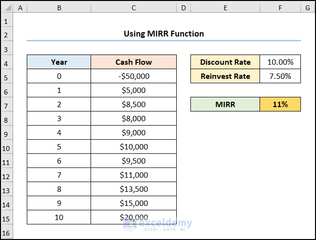
Consider the Yearly Cash Flow of Project Alpha dataset shown in the B4:C15 cells. The dataset shows the Year starting with 0 (Initial investment), the yearly Cash Flows, the Discount Rate of 10%, and the Reinvest Rate of 7.5%.
Example 1 – Calculating MIRR of an Investment
Steps:
- Go to the F7 cell and insert the formula given below.
=MIRR(C5:C15,F4,F5)
The C5:C15 range of cells refers to the Cash Flows, the F4 cell points to the Discount Rate, and the F5 cell indicates the Reinvest Rate.
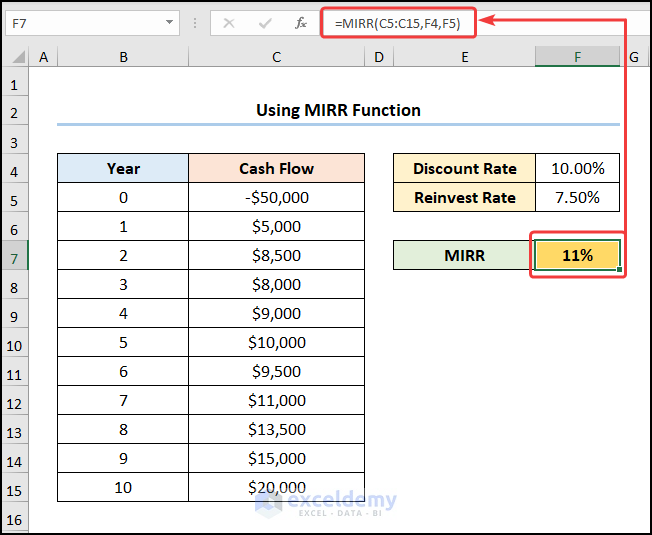
- Hit Enter.
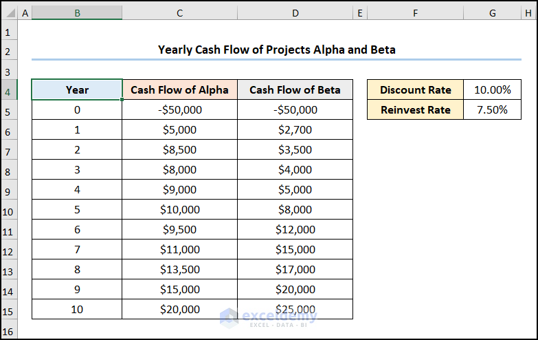
Example 2 – Comparing Two Investments with the MIRR Function
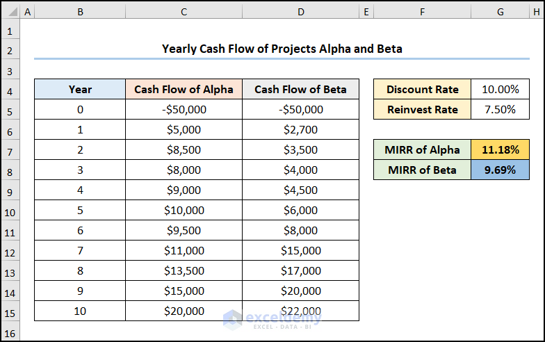
Consider the Yearly Cash Flow of Projects Alpha and Beta dataset shown in the B4:D15 cells. We want to compare the Modified Internal Rate of Return of the two projects to determine which is more profitable.
Steps:
- Go to the G7 cell and enter the expression given below.
=MIRR(C5:C15,G4,G5)
The C5:C15 range of cells refers to the Cash Flows, while the G4 and G5 cells represent the Discount Rate and Reinvest Rate.
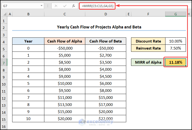
- This returns the Modified Internal Rate of Return of Project Alpha, in this case, it is 11.18%.
- Go to the G8 cell and calculate the Modified Internal Rate of Return of Project Beta which is 9.69%.
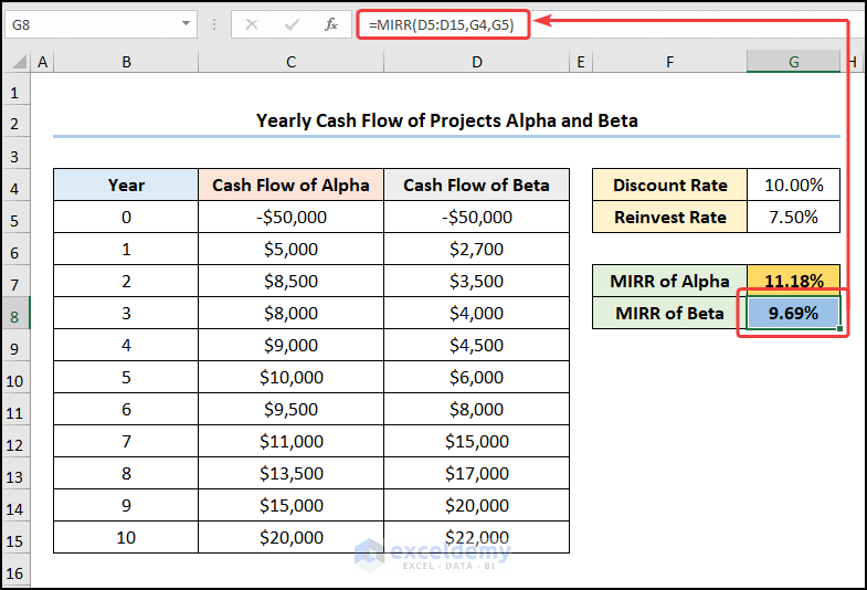
The results should look like the picture shown below, and since the MIRR of Project Alpha is greater than Beta, it is more profitable.
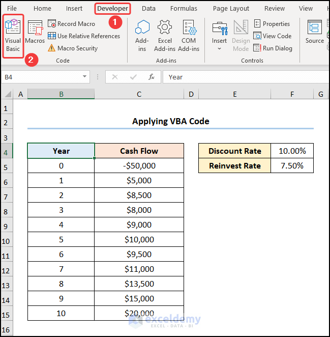
Example 3 – Applying VBA Code
Steps:
- Navigate to the Developer tab and click the Visual Basic option.
This opens the Visual Basic Editor in a new window.
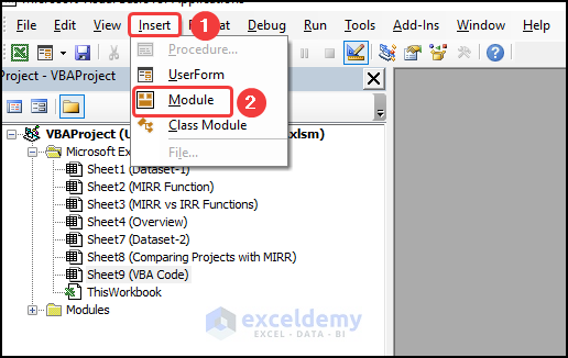
- Go to the Insert tab and select Module.
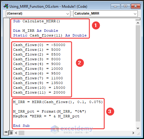
- You can copy the code from here and paste it into the window as shown below.
Sub Calculate_MIRR()

Dim M_IRR As Double
Static Cash_flows(11) As Double

Cash_flows(0) = -50000
Cash_flows(1) = 5000
Cash_flows(2) = 8500
Cash_flows(3) = 8000
Cash_flows(4) = 9000
Cash_flows(5) = 10000
Cash_flows(6) = 9500
Cash_flows(7) = 11000
Cash_flows(9) = 13500
Cash_flows(10) = 15000
Cash_flows(11) = 20000

M_IRR = MIRR(Cash_flows(), 0.1, 0.075)

M_IRR_pct = Format(M_IRR, "0%")
MsgBox "MIRR = " & M_IRR_pct

End Sub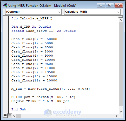
⚡ Code Breakdown:
- The sub-routine is given a name, which is Calculate_MIRR().
- We defined the variables M_IRR, and Cash_Flows and assign the data type Double.
- We entered all the Cash flows manually.
- We used the MIRR function to compute the value and format it as a percentage using the Format function.
- We display the results in the MsgBox function.
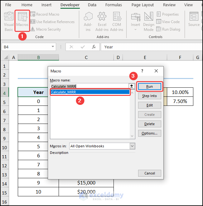
- Close the VBA window and click the Macros button.
This opens the Macros dialog box.
- Select the Calculate_MIRR macro and hit the Run button.
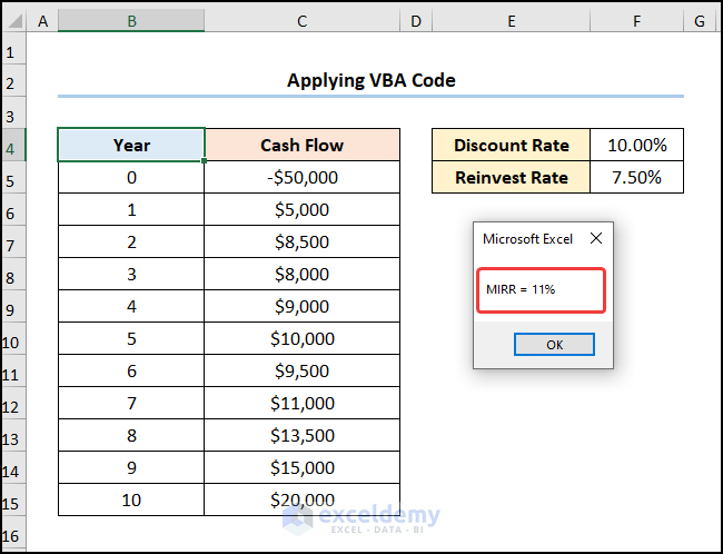
The results should look like the screenshot given below.
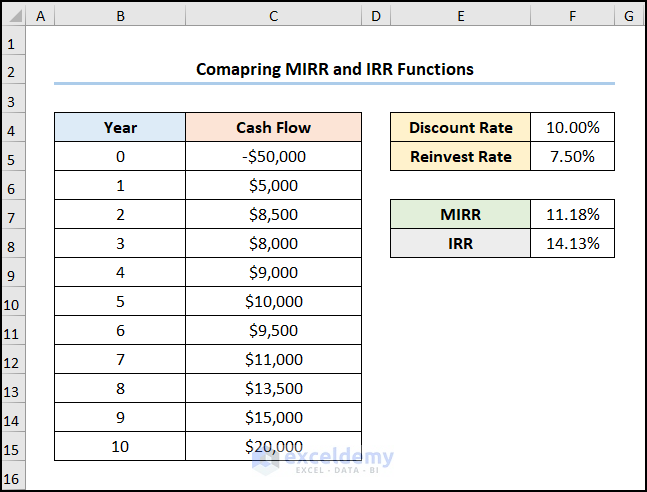
Comparing MIRR and IRR Functions
Steps:
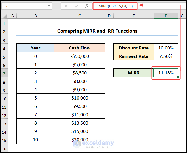
- Jump to the F7 cell and insert the formula below.
=MIRR(C5:C15,F4,F5)
The C5:C15 range of cells refers to the Cash Flows, the F4 cell points to the Discount Rate, and the F5 cell indicates the Reinvest Rate.
- Go to F8 and compute the IRR using the expression given below.
=IRR(C5:C15)
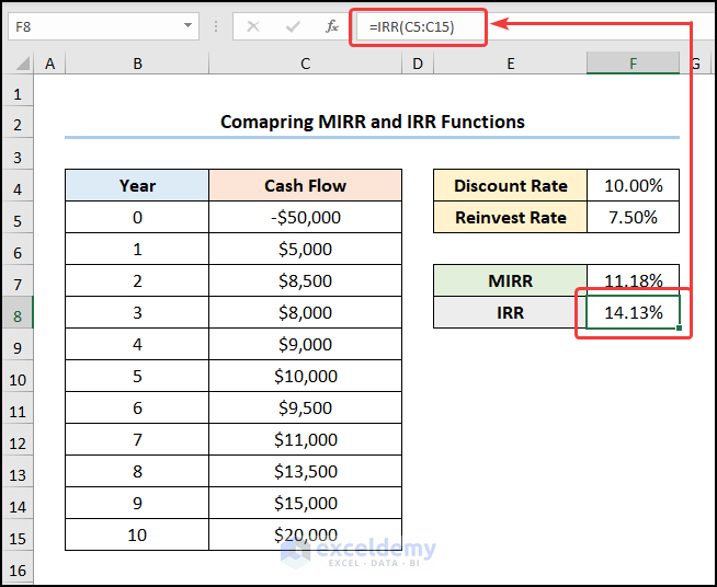
We can see that the IRR of the project is greater than the MIRR which is an overly optimistic estimation of the profitability.
Shortcomings of MIRR Function
Because a project’s earnings are not always fully reinvested, the MIRR function generates a less predictable rate of return. Nevertheless, by changing the reinvest rate, you can compensate for the partial investments.
Things to Remember
- A #DIV/0! error results if the values don’t have at least one positive number (referring to the cashflows) and one negative number (indicating the initial investment).
- The #VALUE! error occurs when one of the arguments, finance rate or reinvest rate, is not a numeric value.
- The MIRR function uses the order of values to determine the order of cash flows under the assumption that all cash flows occur at regular intervals and at the end of each year.
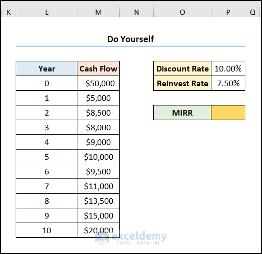
Practice Section
We have provided a Practice section on the right side of each sheet so you can practice.
Download the Practice Workbook
<< Go Back to Excel Functions | Learn Excel
Get FREE Advanced Excel Exercises with Solutions!

Hi, thanks for the article,
If your net income cash flows are already diminished of the interests to be paid, should we put a value for the “finance rate”, or simply 0 to avoid double counting?
Thanks !
Laurene
Hi Laurene,
Thanks for staying with us. If the net income cash flows reduced, or 0 or negative, whatever it is. The value of the argument finance rate doesn’t depend on it. You must give the rate as input which is paid by you for cash flows. When you select the payment and incomes at specified intervals as the Values argument, the finance rate as the rate paid by you for your income, and finally the reinvestment rate, the MIRR function will calculate the rate by automatically adjusting the values.