Mileage reimbursement calculation is one of the most common tasks in a business. You may also know mileage reimbursement as claim cost, or vehicle running cost. In Microsoft Excel, you can do such types of tasks in bulk and within seconds. This article demonstrates a step-by-step guide for how to calculate mileage reimbursement in Excel.
What Is Mileage Reimbursement?
Mileage reimbursement means the amount of money a company owes to an employee after he or she has used his or her personal vehicle for business purposes. It is calculated on the basis of miles, or the distance traveled for a trip.
Arithmetic Formula to Calculate Mileage Reimbursement
The arithmetic formula to calculate mileage reimbursement is as follows:
MR=D*R
In this formula,
- MR = The amount of mileage reimbursement owed to an employee.
- D = Total distance traveled due to business purpose.
- R = Mileage reimbursement rate.
The mileage reimbursement rate may vary in different states or countries.
3 Steps to Calculate Mileage Reimbursement in Excel
Using Microsoft Excel is one of the fastest and most convenient ways to calculate your mileage reimbursement. Now, suppose you need to calculate mileage reimbursement for an employee. Hence, I will show you a step-by-step guide to calculate the Mileage Reimbursement for the employee.
🔷Step 01: Making an Outline to Calculate Mileage Reimbursement
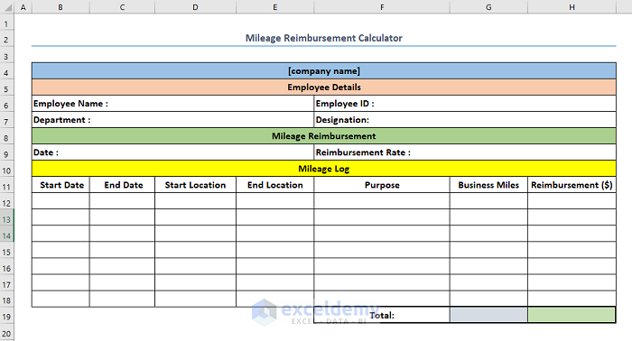
- First, you need to make an outline for the Mileage Reimbursement Calculator.
- In this case, I have shown you an example of an outline.
Also, here I have added Employee Details, Mileage Reimbursement, and Mileage Log for a detailed and efficient Mileage Reimbursement Calculator.
Read More: How to Convert Percentage to Basis Points in Excel
🔷Step 02: Inserting Necessary Data into Excel
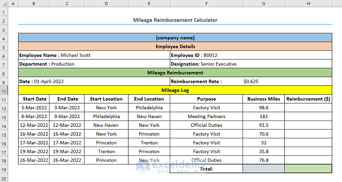
- Second, insert the necessary data into the sheet.
- In this case, I have inserted the following data: Employee Name, Employee ID, Department, Designation, Date, Reimbursement Rate, Start Date, End Date, Start Location, End Location, Purpose, and Business Miles.
Read More: How to Calculate Profitability Index in Excel
🔷Step 03: Calculating Mileage Reimbursement in Excel
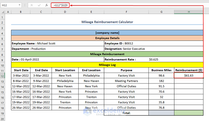
- Third, you need to build a Mileage Reimbursement Calculator.
- Now, for this case, select cell H12 and insert the following formula.
=G12*$G$9Here, cell H12 represents the Reimbursement Rate. Also, cells G12 and G9 indicate the first cell of the columns Business Miles and Reimbursement ($) respectively.
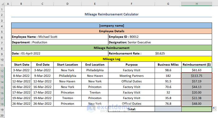
- At this point, drag the Fill Handle for the rest of the cells to the column Reimbursement ($).
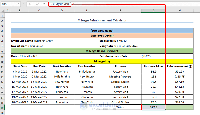
- Next, select cell G19 and insert the following formula.
=SUM(G12:G18)In this case, cell G19 represents the cell for Total Business Miles. Also, cells G12 and G18 indicate the first and last cell of the column Business Miles respectively.
Moreover, here we used the SUM function. The syntax of this function is SUM (number1, [number2], [number3], …).
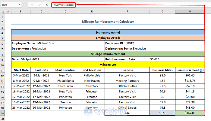
- Finally, select cell H19 and insert the following formula.
=SUM(H12:H18)In this case, cell H19 represents the cell for Total Reimbursement ($). Also, cells H12 and H18 are the first and last cells of the column Reimbursement ($).
Read More: How to Use Macaulay Duration Formula in Excel
💡Things to Remember
- During creating the outline, you can select the format of the cells in the column representing dates in your required date format.
- Also, you can select the format of the Reimbursement Column in your required currency format.
- In this case, you can also calculate the total reimbursement by multiplying cell G19 and the Reimbursement Rate. So, the formula will be as follows:
=G19 * $G$9You can download the practice workbook from the link below.
Conclusion
In this article, you get both a calculator and a template for mileage reimbursement calculations. So, you can download the Template and utilize it as a Mileage Reimbursement Calculator if you want. Last but not least, I hope you found what you were looking for in this article. If you have any queries, please leave a comment below.
Related Articles
- How to Calculate Tracking Error in Excel
- How to Calculate WACC in Excel
- Excel XNPV vs NPV: Comparison with Examples
- How to Calculate Time Weighted Return in Excel
- XIRR vs IRR in Excel
<< Go Back to Excel Formulas for Finance | Excel for Finance | Learn Excel
Get FREE Advanced Excel Exercises with Solutions!
