How to Use Macaulay Duration Formula in Excel (2 Easy Methods)

In this article, I will show you how to use the Macaulay Duration formula in Excel. While performing many financial calculations, especially while dealing with bond/stock calculation, Macaulay Duration is a very significant parameter. Here, we will use a built-in function and a mathematical formula two determine Macaulay Duration in two different circumstances. So, let’s start.

Table of Contents hide

Download Practice Workbook

What Is Macaulay Duration?

2 Useful Methods to Calculate Macaulay Duration in Excel

1. Use of DURATION Function to Calculate Macauly Duration in Excel

2. Application of Mathematical Formula to Calculate Macaulay Duration in Excel

Things to Remember

Conclusion

Download Practice Workbook

Download this practice workbook to exercise while you are reading this article.

Macaulay Duration.xlsx

What Is Macaulay Duration?

Macaulay Duration is a measure of the average time, in years, that it takes for a bond to receive the present value of its cash flows. It is named after Frederick Macaulay, who developed the concept in 1938. The Macaulay Duration is often used to measure the sensitivity of a bond’s price to changes in interest rates. A bond with a longer duration will experience larger price changes in response to changes in interest rates. Conversely, a bond with a shorter duration will experience smaller price changes in response to changes in interest rates. The Macaulay Duration can be used to compare bonds with different maturities, coupons, and frequencies of interest payments. It is a useful tool for investors who want to manage the risk of their bond portfolios by understanding how sensitive the bonds are to changes in interest rates.

2 Useful Methods to Calculate Macaulay Duration in Excel

In this section, we will demonstrate 2 effective methods to calculate Macaulay Duration in Excel with appropriate illustrations. In the first method, we will use the DURATION function. On the other hand, in the 2nd method, we will apply a mathematical formula for a special case. So, let’s explore the methods one by one.

1. Use of DURATION Function to Calculate Macauly Duration in Excel

In this method, we will get familiar with the built-in DURATION function of Excel to calculate the Macaulay Duration. For illustration purposes, I have taken an example where we have the following parameters: Annual Coupon Rate, Yield Rate, Settlement Date, Maturity Date, Payment Frequency, and Basis. (Shown the figure below).

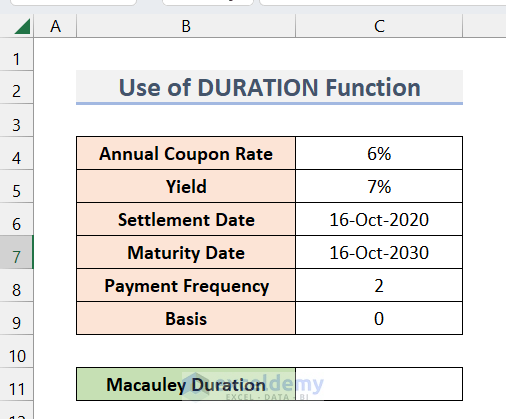
And now, we want to calculate the Macaulay Duration. To do that, follow the steps below.

Steps:

First, select cell C11 and write down the following formula.

=DURATION(C6,C7,C4,C5,C8,C9)

Here,

C6 is the Settlement Date (The settlement date of a bond is the date on which the bond is transferred from the seller to the buyer)

C7 is the Maturity Date (It is the date on which the principal amount of the bond is due to be repaid to the bondholder)

C4 is the Annual Coupon Rate (It is the amount of interest that a bond pays per year, expressed as a percentage of the face value)

C5 is the Yield (The yield of a bond is the rate of return that an investor will earn by holding the bond until it matures)

C8 is the Payment Frequency (Number of times payment will be made)

C9 is the Basis ( This argument counts how the days are counted. 0 is for US 30/360 )

Now, click Enter and you will see the result.

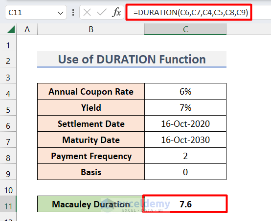
So, here, we can see that the Macaulay Duration is 7.6 Years in this case.

In this way, we can easily calculate the Macaulay Duration for similar situations like this.

2. Application of Mathematical Formula to Calculate Macaulay Duration in Excel

In this method, we will use some custom formulas to calculate the Macaulay Duration in multiple steps. For illustration, I have taken an example data set with the following specifications.

Here, we need to input the Maturity time directly, unlike the first method where we need to separately give the Settlement and Maturity Dates. Moreover, we also have the Face value of the bond (100). On the other hand, in method 1, Face value has always a unstated default value of 100. Now, we will determine the Macaulay Duration in the following steps.

Steps:

First of all, we will calculate the price of the bond. To do that, write the following formula in cell C9 and press Enter.

=(((C4*C8)/C6)*((1-(1/(1+(C5/C6))^(C7*C6))))/(C5/C6))+(C8/((1+(C5/C6))^(C7*C6)))

Here, the formula that we have used is

Where,

r = Yield rate/ Frequency

n= Frequency * Face Value

As a result, we will get the value of the bond price.

Now, we will calculate the Macaulay Duration of the bond using the price of the bond. To do that, write down the following formula in cell C11 and press OK.

=((((C4*C8)/C6)/((C5/C6)^2)*((1-(1/(1+(C5/C6))^(C7*C6)))))+(C7*C6*(C8-((C4*C8/2)/(C5/C6)))/((1+(C5/C6))^((C7*C6)+1))))/C10/C6*(1+(C5/C6))

The formula that we used to calculate Macaulay Duration is,

Where,

t = time period

C = coupon payment

y = yield

n = number of periods

M = maturity

Consequently, you will get the Macaulay Duration which is precisely the same as the previous method.

By using the given template file, you can directly input your values and get the Macaulay Duration accordingly.

Things to Remember

In method 1, we can directly pass the arguments of the DURATION function. Though we recommend using cell references in the arguments, especially for date-type values.

Conclusion

That is the end of this article regarding how to use the Macaulay Duration formula in Excel. If you find this article helpful, please share this with your friends. Moreover, do let us know if you have any further queries. Finally, please visit Exceldemy for more exciting articles on Excel.