How to Use the XIRR Function in Excel (3 Methods)

The following dataset has Periods, Cash Flow, and Date columns. Using this dataset, we will show 3 methods for using the XIRR function in Excel.

Method 1 – Using the Basic XIRR Function

Steps:

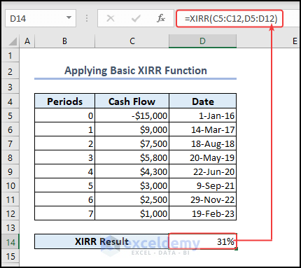
Enter the following formula in cell D14:

=XIRR(C5:C12,D5:D12)

Press ENTER.

The internal rate of return is in cell D14.

Method 2 – Applying the XIRR Function with Initial Guess

Steps:

For this dataset, the XIRR function without the guess of the initial rate of return, returns an error. If we can guess the initial rate of return, then using it will help us avoid this error.

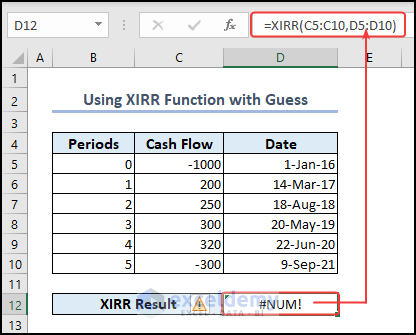
Enter the following formula in cell D14:

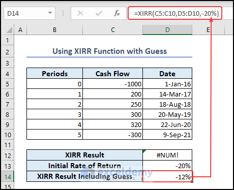
=XIRR(C5:C10,D5:D10,-20%)

Here,

-20% is the Guess, which is the initial rate of return as the third argument of the function.

Press ENTER.

A value of –12% is returned in cell D14.

The anticipated return rate (-20%) used as a guess argument helps the XIRR function to arrive at the result.

Method 3 – Using the XIRR Function for Monthly Cash Flows

Steps:

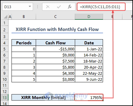
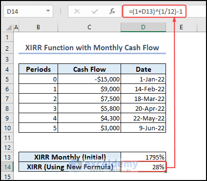
Enter the following formula in cell D14 to find the monthly IRR:

=(1+D13)^(1/12)-1

Press ENTER.

You can see the monthly IRR in cell D14.

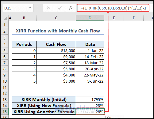
Another way to find the monthly IRR is to insert the XIRR function directly in the equation.

Enter the following formula in cell D15:

=(1+XIRR(C5:C10,D5:D10))^(1/12)-1

Press ENTER.

You can see the monthly IRR in cell D15.

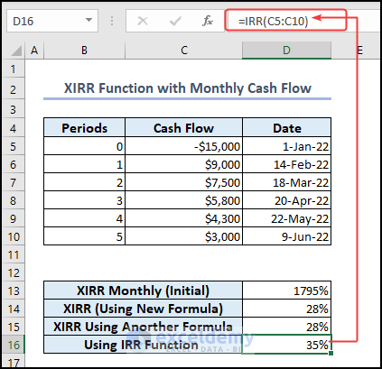
We can also use the IRR function to learn the monthly IRR.

Enter the following formula in cell D16:

=IRR(C5:C10)

Press ENTER

You will see the monthly IRR in cell D16.

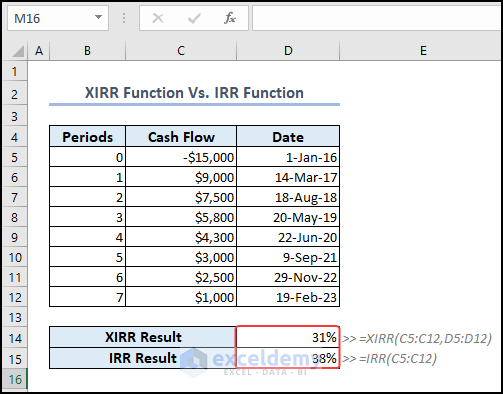
XIRR Function vs. IRR Function in Excel

Here, we will describe the difference between XIRR and IRR functions.

XIRR Function: The XIRR function lets you specify a date for each cash flow. You can compute the IRR for cash flows that don’t occur at regular intervals.

IRR Function: The IRR function presumes that each period within a sequence of cash flows is of equal length. This function is suitable for computing the IRR for cash flows that occur regularly, such as on a monthly, quarterly, or annual basis.

When the precise dates of cash payments are known, the XIRR function is recommended. This is because it offers more accurate calculations.

When cash payments are made at fixed and consistent intervals, the results returned by the functions are similar.

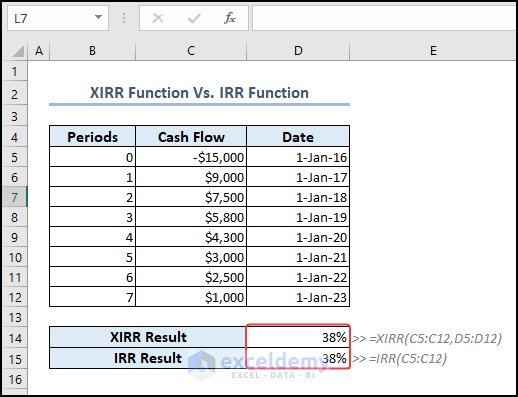
For a non-periodic cash flow, there can be a substantial difference between the results produced by the functions.

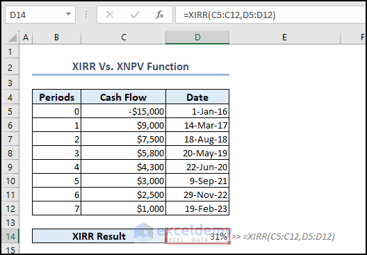
XIRR Function Vs. XNPV Function in Excel

The XIRR function computes the IRR for cash flows that don’t occur at regular intervals. On the other hand, the XNPV function finds out the present value of a set of cash flows at a fixed rate of return.

XIRR and XNPV are closely connected functions. The interest rate corresponding to XNPV = 0 is the rate of return computed by XIRR.

In the following picture, you can see the XIRR result in cell D14.

We have used the following formula to find the IRR value in cell D14.

=XIRR(C5:C12,D5:D12)

After pressing ENTER, we get the output in cell D14.

Now, it’s time to determine the XNPV result. We need a discount rate to do this.

Here, we take a 15% discount rate in cell D15.

We enter the following formula in cell D15.

=XNPV(D15,C5:C12,D5:D12)

After pressing ENTER, we can see the XNPV Result in cell D15.

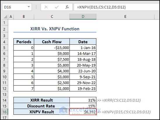
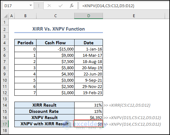
Now, if we use the XIRR Result as the discount rate, which is 31% instead of 15%, we will get the XNPV value as 0.

To show this, we type the following formula in cell D16.

=XNPV(D14,C5:C12,D5:D12)

Here, D14 is the XIRR Result, which is 31%.

Then, we press ENTER.

Thus, you can see the XNPV Result is 0.

XIRR Function is Not Working in Excel

If your XIRR function is not working, consider the following key factors to investigate.

#NUM! Error

The following reasons are responsible for a #NUM! error.

The number of columns or rows for the Cash Flows and date ranges are not equal in length.
The cash flow column does not contain at least one incoming (+) and one outgoing (-) cash flow.
Any of the following dates are before the starting date.
A solution is not reached within 100 iterations. In this case, try using an alternative guess.

#VALUE! Error

The following reasons are responsible for a #VALUE! error.

Cash flow values are not numeric.
Dates are not input as valid dates.

Things to Remember

The XIRR function calculates the internal rate of return for a series of cash flows that occurred at irregular intervals.
The first payment is optional and corresponds to a cost or payment that occurs at the beginning of the investment. If the first value is a cost or payment, it must be a negative value.
Payments are expressed as positive values. All succeeding payments are discounted based on a 365-day year.