How to Calculate Volatility in Excel (2 Suitable Ways)

What Is Volatility?

Volatility is the measure of the fluctuations of return of any stock or security over a time period. It is calculated based on the standard deviation or variance of returns over a time period. In the financial market, when the stock index increases or decreases more than 1% over a limited time, that is called a volatile market.

Types of Volatility:

• Historical Volatility:

This calculates volatility based on past information. It predicts the future by analyzing past values. It does not consider future trends, market conditions, or needs. But It is not forward-looking. It is also called historical volatility.

• Implied Volatility:

The implied volatility is forward-looking. It does not care the past performance and considers future expectations. It is also called projected volatility.

How to Calculate Volatility in Excel? (Both Historical and Implied Volatility)

Method 1 – Calculating Historical Volatility in Excel

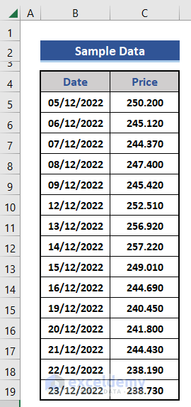
We will collect stock data from Yahoo Finance.

Steps:

• We collected the following sample data.

• We added a row on the right side.
• Use the following formula on cell D6.

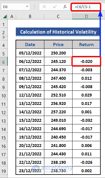
We compared the price of the present day with the previous day and subtracted 1. We can also use the following formula based on the LN function.

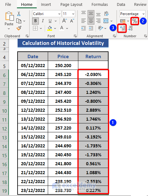
• Select range D6:D19.
• Choose Percentage from the Number group of the Home tab.

• Add two new columns to the dataset.

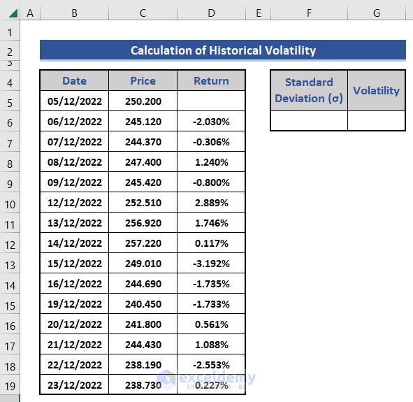
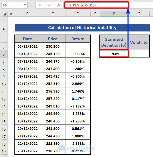
• Put the following formula in cell F6 for standard deviation.

• Use the standard deviation to calculate volatility. Apply the following formula in cell G6.

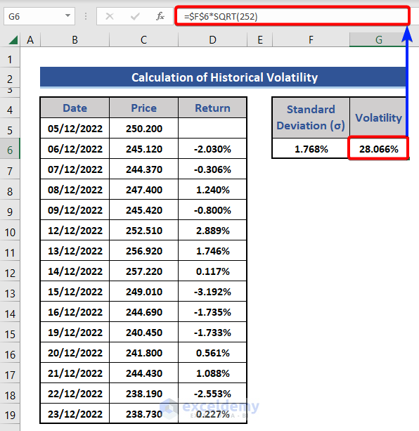
We calculated the historical volatility. This volatility is also called annualized volatility as we used 252 in the equation. Here, the value of standard deviation is also called daily volatility. If we want to get monthly volatility, we need to use 22. The formula will look like this:

Method 2 – Calculating the Implied Volatility

To calculate implied volatility, we need to follow the Black Scholes Model:

Steps:

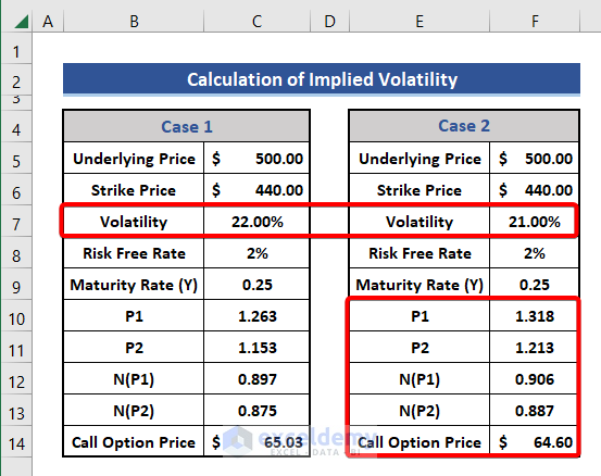
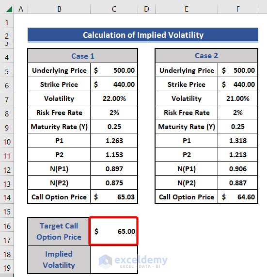
• Insert data on Underlaying Price, Strike Price, Volatility, Maturity Time, and Risk-Free-Rate in the dataset for two cases.

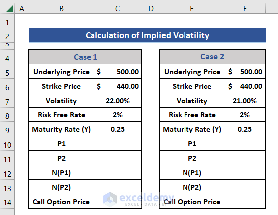
• The value of volatility is different in the two cases, and the rest are the same.
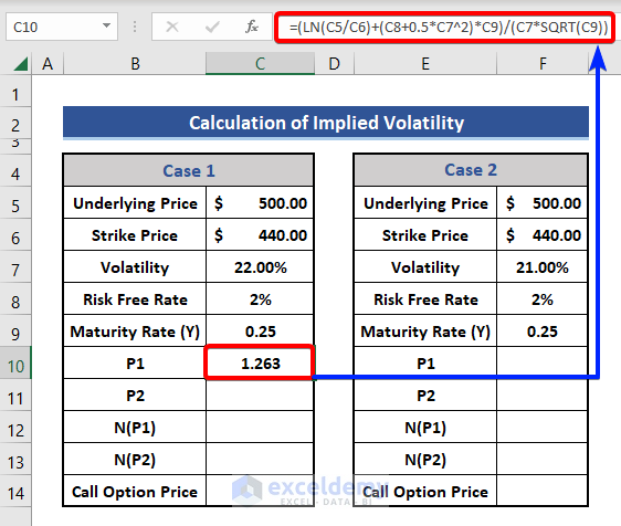
• Calculate conditional probability P1 using the following formula.

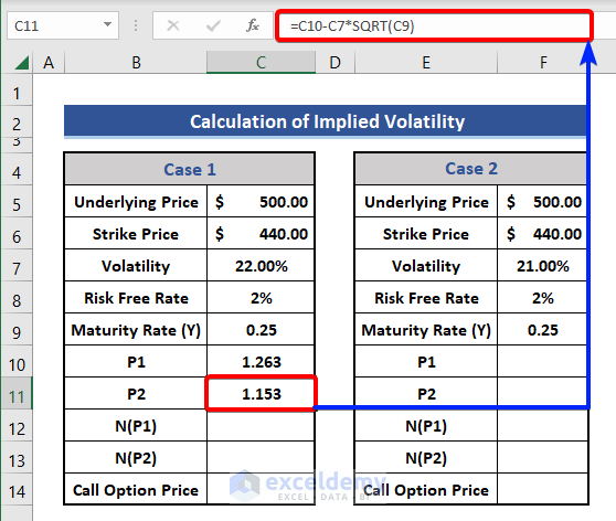
• Use the SQRT function to calculate probability P2.

• Calculate the normalized distribution on cells C12 and C13 using the following formulas:

For Cell C12:

For Cell C13:

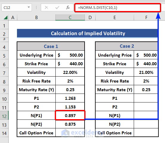
• Use the NORM.S.DIST function to calculate the normal distribution for N(P1) and N(P2).
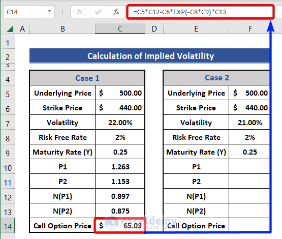
• Calculate the Call Option Price using this formula:

• Repeat for Case 2.

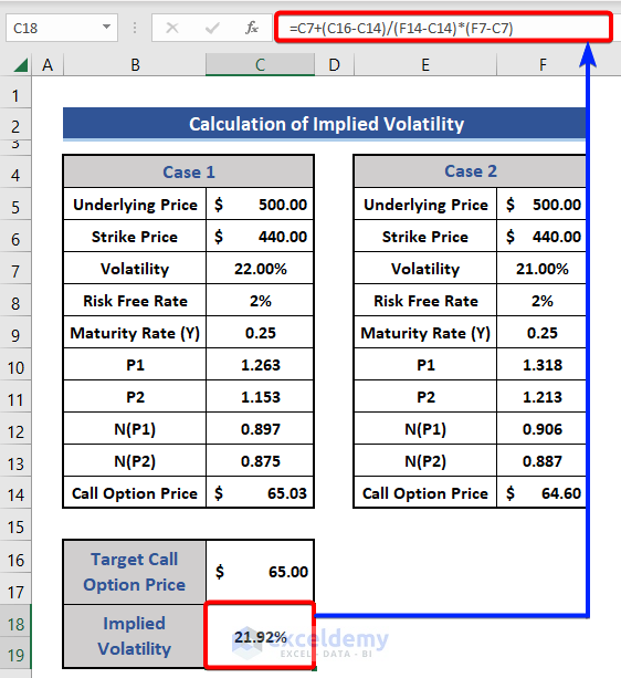
• Add two new rows and set the Target Call Option Price to $65.

• Use the following formula to get the implied volatility based on the Black Scholes Model.

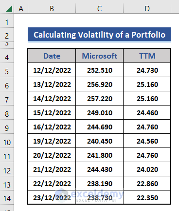
How to Calculate the Volatility of a Portfolio in Excel

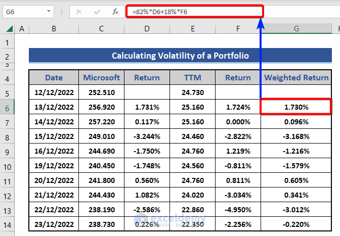
We will consider the closing stock price of Microsoft and Tata Motors for the last 10 days. The weight of Microsoft is 82%, and Tata Motors is 18%.

Steps:

• Insert data from Microsoft and Tata Motors into the dataset.

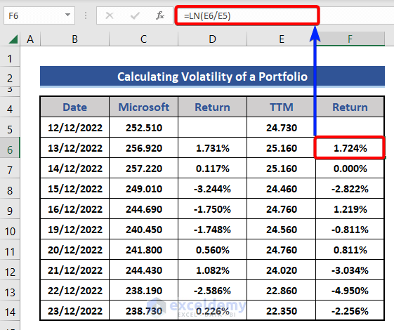
• Add two new columns in the dataset for calculating returns.
• Apply the formulas based on the LN function to get a return.

For Cell D6:

For Cell F6:

• Calculate the weighted return with the following formula:

• Add a new row 16 in the dataset for Portfolio Volatility.
• Insert the following formula in cell D16.

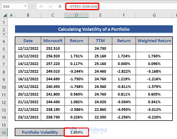
This is also called the daily portfolio volatility. If we want monthly or annualized volatility, we need to multiply by the square root of 22 and 252, respectively.

Download the Practice Workbook

Volatility In Excel: Knowledge Hub

• How to Calculate Volatility for Black Scholes in Excel
• How to Calculate Realized Volatility in Excel
• How to Generate Volatility Surface in Excel

<< Go Back to Excel for Finance | Learn Excel