Undoubtedly, Excel’s ability to crunch numbers and plot three-dimensional graphs can help us better understand and represent the volatility of stocks. With this in mind, this article shows the process of how to generate volatility surface in Excel in detail.
What Is Volatility Surface?
In a nutshell, the Volatility Surface is a three-dimensional representation of “Time” to maturity, the “Strike” price, and the “Implied Volatility”. Ideally, the implied volatility surface should be plain, however, in practice, it is usually curved due to limitations in the Black-Scholes model.
As a note, we’ll use the Dumas, Fleming, and Whaley specifications to model Implied Volatility using the formula given below.
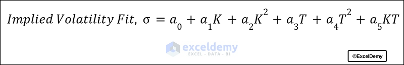
where,
- K is the Strike price
- T is the Time to maturity in Years
- a0, a1, a2, a3, a4, and a5 are the Coefficients
How to Generate Volatility Surface in Excel: with Detailed Steps
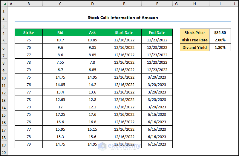
First of all, let’s suppose the Stock Calls Information of Amazon shown in the B4:F19 cells. Here, the dataset depicts the “Strike” price, “Bid” and “Ask” prices, “Start Date”, and “End Date” columns. In addition, we have the “Stock Price”, “Risk-Free Rate”, and “Div & Yield” percentages. So, without further delay, let’s see each step on how to generate a volatility surface in Excel with the necessary illustrations.
Here, we have used the Microsoft 365 version; you may use any other version according to your convenience.
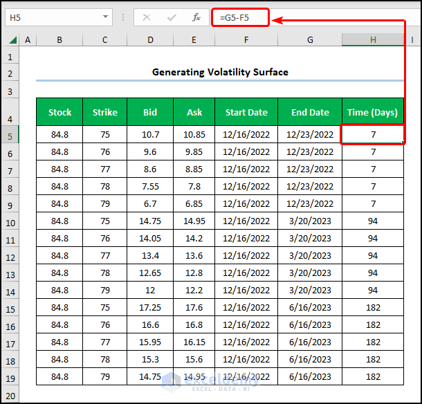
📌 Step 1: Calculate Time to Maturity
- First, go to the H5 cell >> subtract the value in the F5 cell from the value in the G5 cell.
=G5-F5
In this case, the F5 and G5 cells indicate the “Start” and “End Dates” respectively.
Read More: How to Calculate Daily Volatility in Excel
📌 Step 2: Obtain Implied Volatility with VBA Code
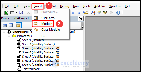
- Second, move to the Developer tab >> click the Visual Basic button.
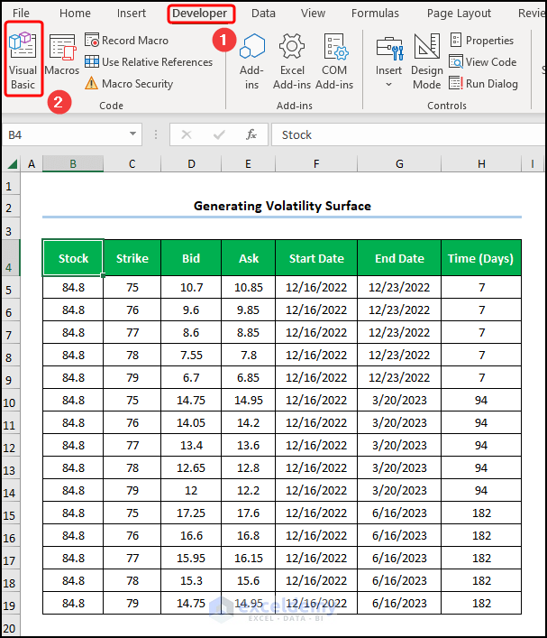
This now launches the Visual Basic Editor in a new window.
- Next, press the Insert tab >> select Module.
For your ease of reference, you can copy the code from here and paste it into the window as shown below.
Function Black_Scholes(Stock_price, Strike, Risk_free_rate, Div_Yield, Sigma_val, Time)

Dim D_1, D_2, n_D_1, n_D_2

    D_1 = (Log(Stock_price / Strike) + (Risk_free_rate - Div_Yield + 0.5 * Sigma_val ^ 2) * Time) / (Sigma_val * Sqr(Time))
    D_2 = D_1 - Sigma_val * Sqr(Time)
    n_D_1 = Application.NormSDist(D_1)
    n_D_2 = Application.NormSDist(D_2)

    Black_Scholes = Exp(-Div_Yield * Time) * Stock_price * n_D_1 - Exp(-Risk_free_rate * Time) * Strike * n_D_2
End Function

Function Bisection_method(Stock_price, Strike, Risk_free_rate, Div_Yield, Time, callmktprice)
    x = 5
    y = 0
    Do While (x - y) > 0.00000001

    If Black_Scholes(Stock_price, Strike, Risk_free_rate, Div_Yield, (x + y) / 2, Time) > callmktprice Then
             x = (x + y) / 2
             Else: y = (x + y) / 2
    End If
    Loop

    Bisection_method = (x + y) / 2
End Function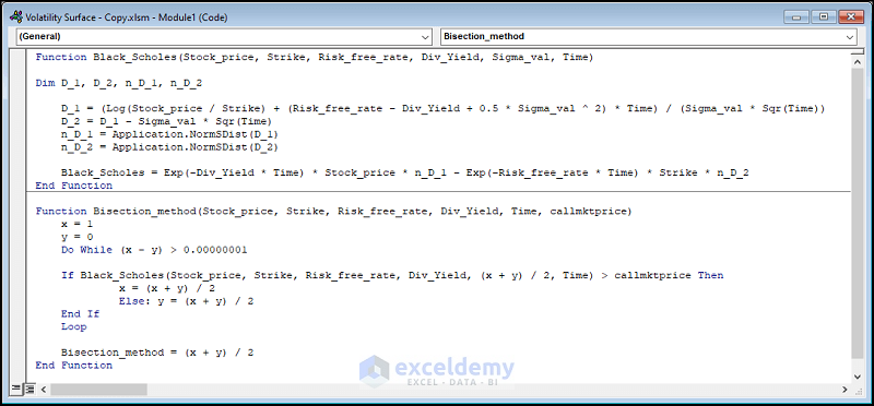
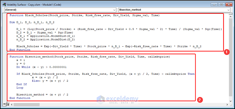
At this point, we’ll explain the VBA code to compute the implied volatility.
- In the first portion, the function is given a name, here it is Black_Scholes() and takes the arguments “Stock_price”, “Strike”, “Risk_free_rate”, “Dive_Yield”, “Sigma_val”, and “Time” to expiry.
- Next, define the variables D_1, D_2, n_D_1, and n_D_2.
- Then, assign the formulas shown below to the D_1 and D_2 variables and use the NormSDist function to the n_D_1, and n_D_2 variables.
- Lastly, enter the expression into the Black_Scholes variable.
- In the later portion, name the function Bisection_method and assign the values 1 and 0 to x and y.
- Following this, combine Do While and If statements to obtain the implied volatility.
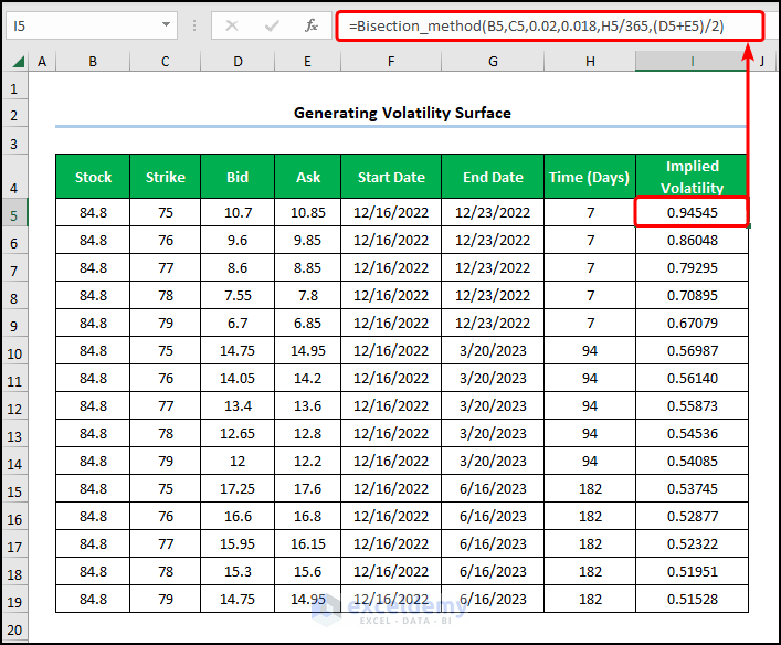
- Not long after, close the VBA window >> call the Bisection_method function to return the “Implied Volatility” >> use the Fill Handle tool to drag the formula to the cells below.
=Bisection_method(B5,C5,0.02,0.018,H5/365,(D5+E5)/2)
For instance, the B5, C5, D5, E5, and H5 cells point to the “Stock”, “Strike”, “Bid”, “Ask”, and “Time” columns respectively.
Read More: How to Calculate Volatility for Black Scholes in Excel
📌 Step 3: Compute the Coefficients for Implied Volatility Fit
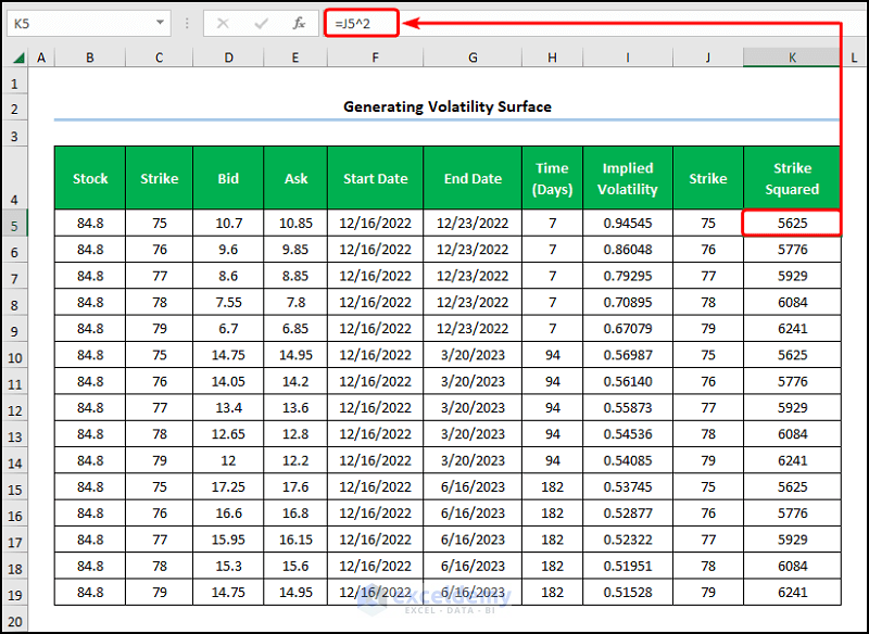
- Third, copy and paste the “Strike” price in column J >> navigate to the K5 cell >> obtain the square of the “Strike” price.
=J5^2
Here, the J5 cell represents the “Strike” price of “75”.
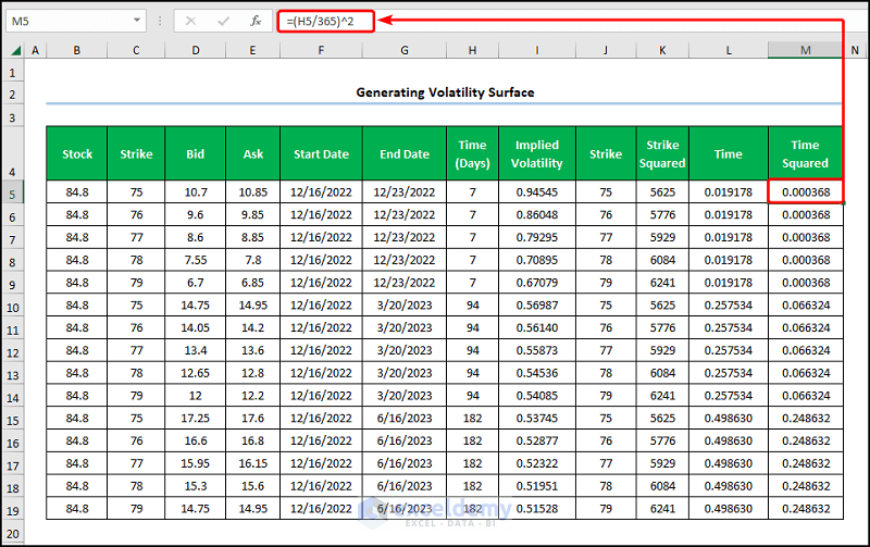
- Now, insert a “Time” column >> get the “Time” in years using the formula below.
=H5/365
In this situation, the H5 cell refers to the “Time” in days, and the “365” is the number of days in a year.

- In a similar style, calculate the “Time” squared value.
=(H5/365)^2
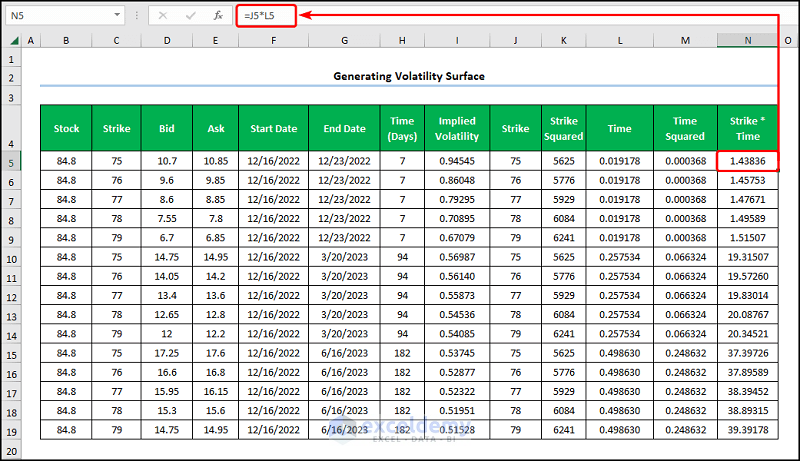
- Afterward, compute the product of the “Strike” and “Time” in the N5 cell.
=J5*L5
In this scenario, the J5 and L5 cells indicate the “Strike” and “Time”.
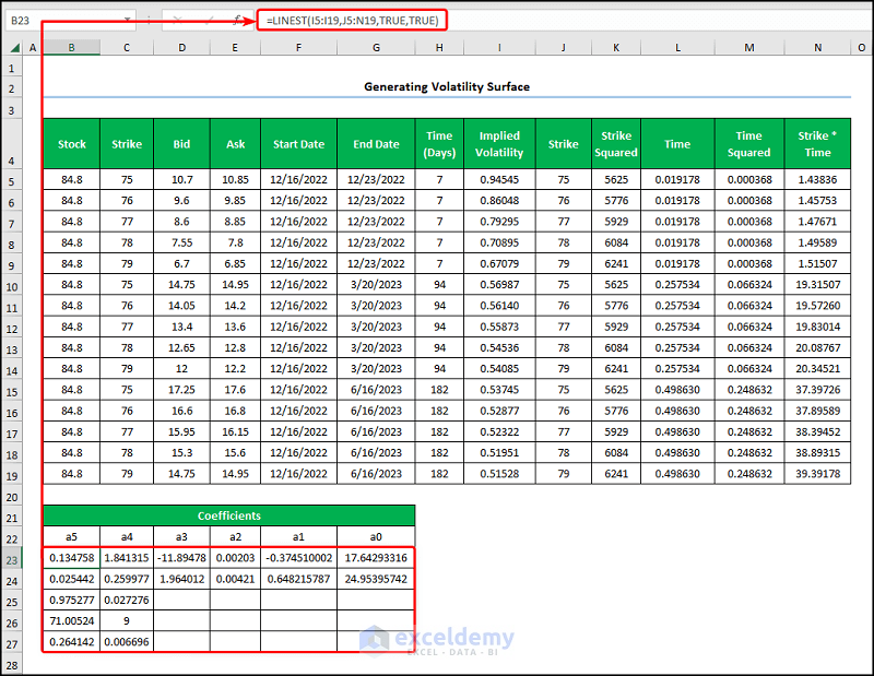
- Consequently, generate the values of the coefficients using the LINEST function.
=LINEST(I5:I19,J5:N19,TRUE,TRUE)
- LINEST(I5:I19,J5:N19,TRUE,TRUE) → returns statistics that describe a linear trend matching known data points, by fitting a straight line using the least squares method. Here, the I5:I19 and J5:N19 are the known_x and known_y arguments that refer to the “Implied Volatility” column and the “Strike”, “Strike Squared”, Time, “Time Squared”, and “Strike*Time” columns respectively. Next, TRUE points to the optional const argument that calculates the constant value normally. Lastly, TRUE represents the optional stat argument which returns additional regression statistics.
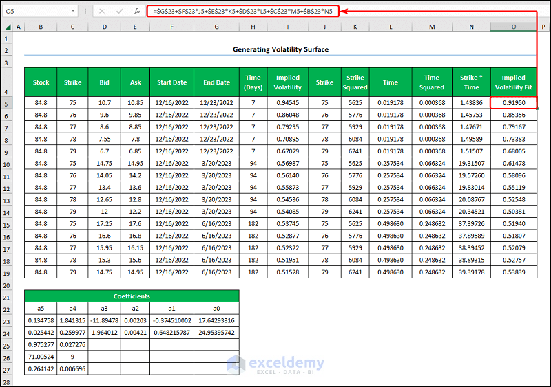
- Lastly, we can calculate the “Implied Volatility Fit” using the Dumas, Fleming, and Whaley equation.
=$G$23+$F$23*J5+$E$23*K5+$D$23*L5+$C$23*M5+$B$23*N5
Now, in the above expression, the G23, F23, E23, D23, C23, B23 cells point to the coefficients “a0, a1, a2, a3, a4, and a5” respectively. Moreover, the J5, K5, L5, M5, and N5 cells represent the “Strike”, “Strike Squared”, Time, “Time Squared”, and “Strike*Time” columns, correspondingly.
📃 Note: Please make sure to use Absolute Cell Reference by pressing the F4 key on your keyboard.
Read More: How to Calculate Implied Volatility in Excel
📌 Step 4: Generate the Table for Volatility Surface
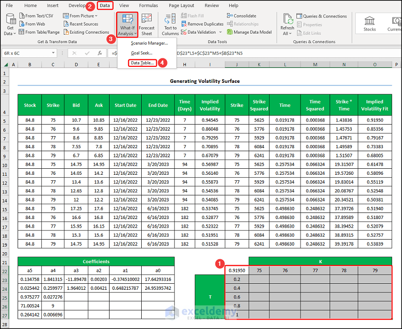
- Fourth, copy and paste the Dumas, Fleming, and Whaley equation into the J22 cell >> construct a table with varying values of “Strike price, K” and “Time, T”.

- Following this, select the J22:O27 cells >> jump to the Data tab >> click What-If Analysis >> choose Data Table.
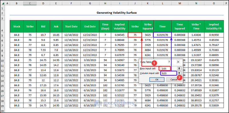
- Next, enter the J5 and L5 cell references as the Row and Column input cells.
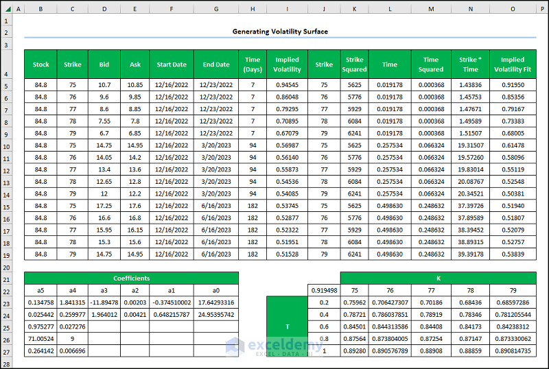
Eventually, the table should resemble the image shown below.
📌 Step 5: Plot Volatility Surface
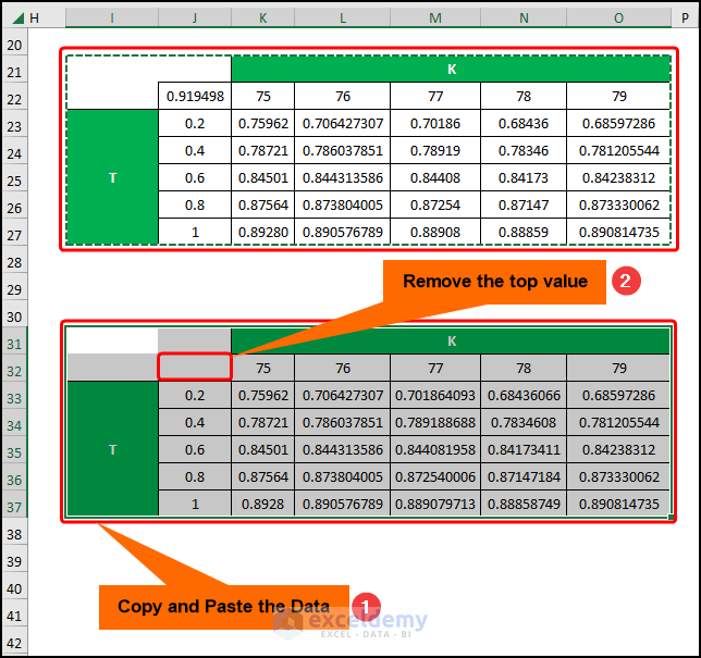
- Fifth, copy the table >> paste it in the I31 cell as shown below >> remove the top value in the J32 cell.
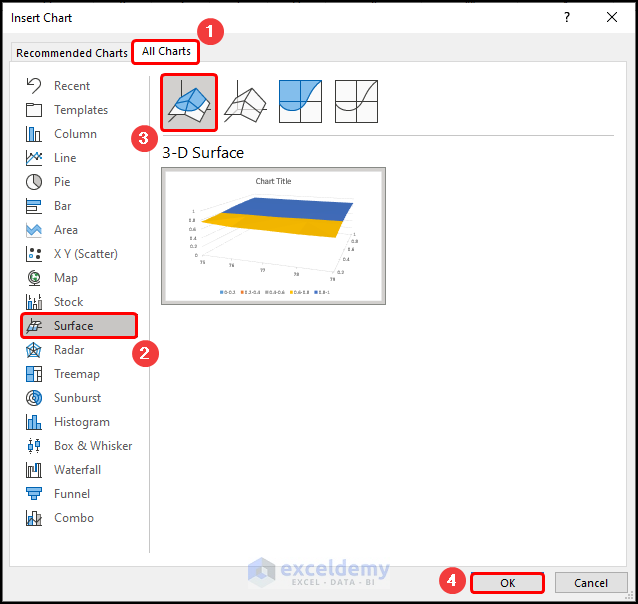
- In turn, choose the J32:O37 cells >> proceed to the Insert tab >> press Recommended Charts.

- At this point, select the All Charts tab >> choose 3-D Surface from the list >> hit the OK button.
- Then, select the chart >> choose a Chart Style according to your preference.
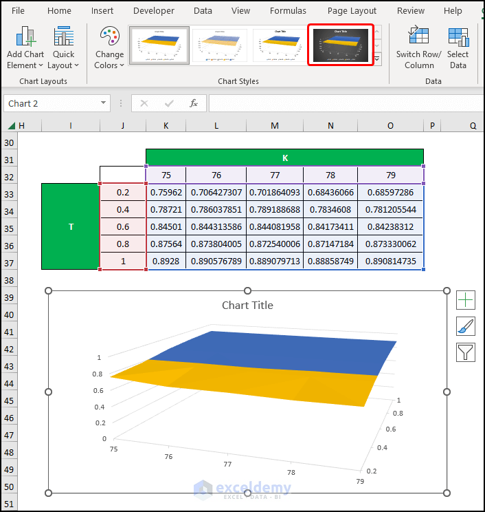
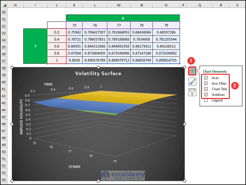
Afterward, format the chart using the Chart Elements option.
- In addition to the default selection, you can enable the Axes Title to provide axes names. Here, it is “Strike”, “Time”, and “Implied Volatility”.
- Now, add the Chart Title, for example, “Volatility Surface”.
- Lastly, you can enable the Gridlines option.
- Furthermore, right-click on the chart >> navigate to 3-D Rotation.
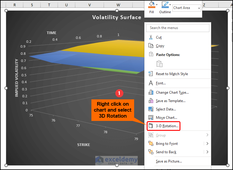
- Next, in the Format Chart Area pane, enter the X and Y Rotations and Perspective values as shown in the picture below.

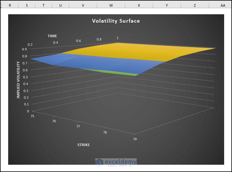
Subsequently, the final output should appear in the figure shown below.
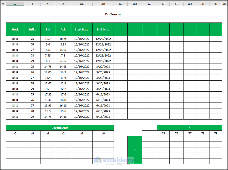
Practice Section
We have provided a Practice section on the right side of each sheet so you can practice yourself. Please make sure to do it by yourself.
Download Practice Workbook
Conclusion
In essence, this article shows a step-by-step guide on how to generate a volatility surface in Excel. So, read the full article carefully and download the free workbook to practice. Now, we hope you find this article helpful, and if you have any further queries or recommendations, please feel free to comment here.
Related Article
- How to Calculate Annualized Volatility in Excel
- How to Calculate Historical Volatility in Excel
- How to Calculate Realized Volatility in Excel
<< Go Back to Volatility In Excel | Excel for Finance | Learn Excel
Get FREE Advanced Excel Exercises with Solutions!
