How to Calculate Historical Volatility in Excel (with Easy Steps)

What Is Historical Volatility?

In business aspects, the monetary value of different financial factors (i.e., stocks and currency) keeps fluctuating because of ins and outs of assets by the traders in the market. This variation over a certain period of time is defined as “Volatility”. Volatility is also an indicator of risk associated with the business.

There are several ways to calculate volatility. But most often, business analysts prefer “Historical Volatility”. Historical Volatility emphasizes previous performances. It provides a long-term assessment of risk associated with the business model. This is widely used for investment strategies. A higher historical volatility is an indicator of greater risk. Even then, some investors look for higher volatility for better profit opportunities.

How to Calculate the Historical Volatility in Excel: with Easy Steps

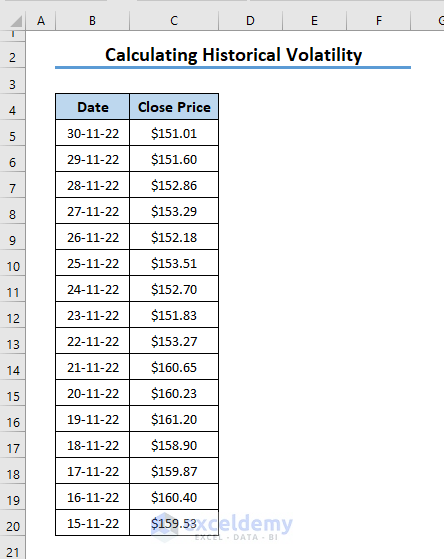
Step 1 – Input Historical Data

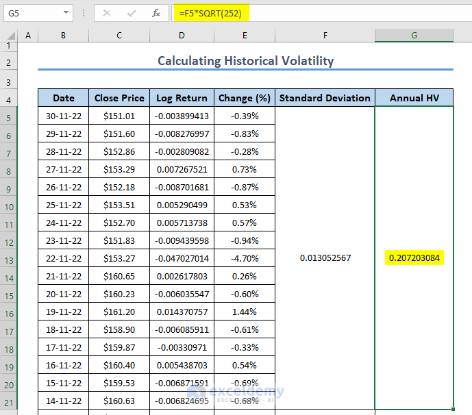
The daily historical closing price and time span (i.e. Date) are used to calculate the daily historical volatility.

We have inserted the historical data in column A and column B of the Excel worksheet. The values are sorted from earliest to oldest dates.

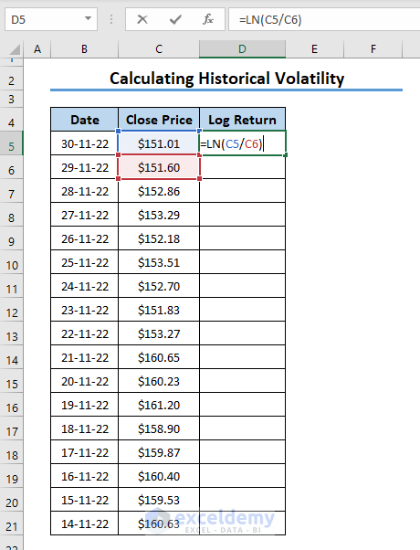
Step 2 – Find the Logarithmic Return

Use the following formula in cell D5:

=LN(C5/C6)

C5 = Closing Price of a particular Date
C6 = Closing Price of the Date before the mentioned date

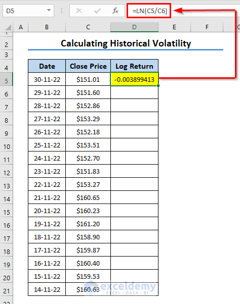
Press Enter and the cell will calculate the log-returns of the dividend of the close price of the date and its previous date.

Drag the Fill Handle tool down to Autofill the formula for the other timeframes.

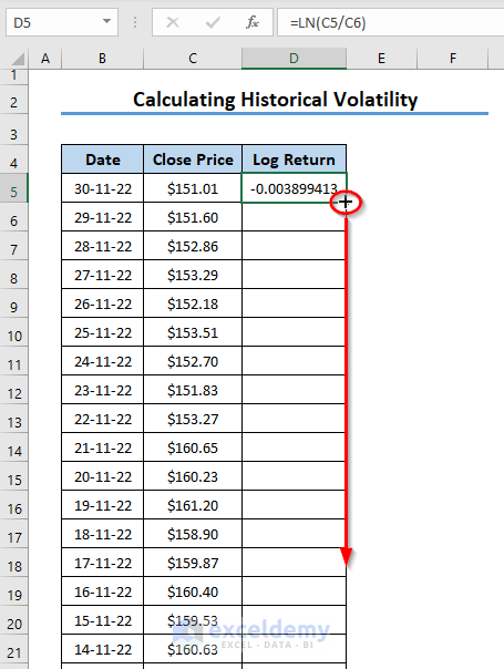
You will find the logarithmic return for all dates.

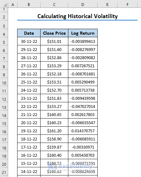
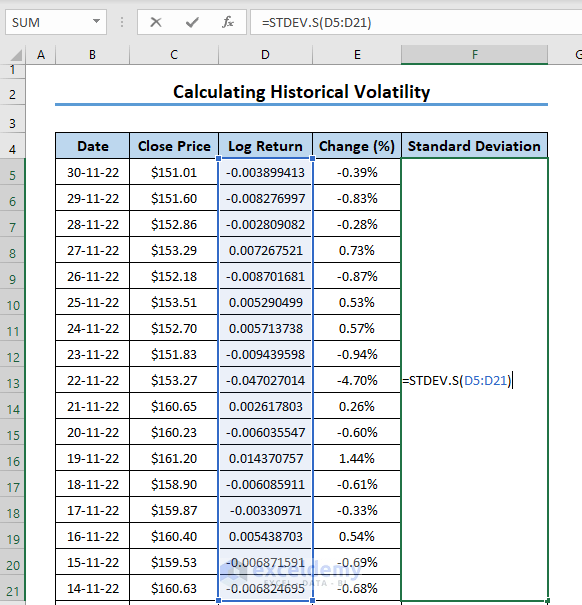
You can show the change of log return in percentage. Create another column, use the return and click the percentage icon from the toolbar.

Step 3 – Calculate the Standard Deviation

Select a cell and apply the following formula in that cell.

=STDEV.S(D5:D21)

D5:D21 is the range of numbers of log-returns.

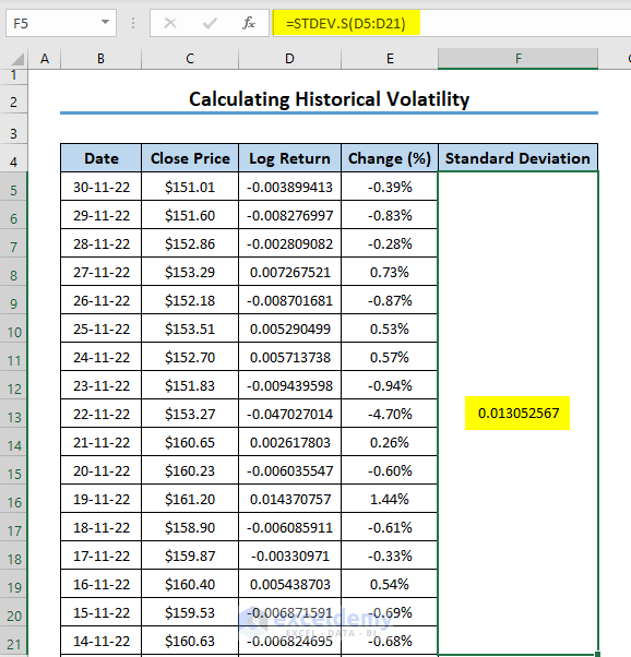
Hit Enter.

Step 4 – Get the Annual Historical Volatility

Select a cell and use the following formula in the selected cell:

=F5*SQRT(252)

F5 = Standard Deviation
252 = Trading Days in a year

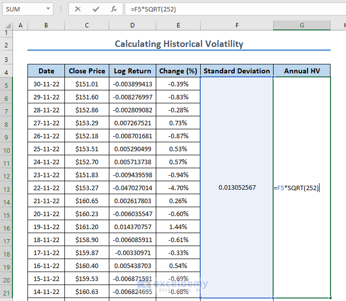
Press Enter.

Things to Remember

Historical volatility gives an idea about the previous performance of a business model.
The risk associated with the security increases with the historical volatility.
Sometimes, higher volatility is sought out by some traders for greater profit and investment opportunities.