When investing in a business or stock market, we need to know how much take we risk or how much profit we can make through this asset. In this regard, the Annualized Volatility calculation is a crucial factor. In this article, I will show you all the quick steps to calculate annualized volatility in Excel.
What Is Annualized Volatility?
Annualized volatility is a statistical measurement of the dispersion of an asset or stock. Generally, it is measured by the standard deviation of the continuously compounded daily return of the asset or stock. The higher the value is, the riskier the investment is.
To calculate this, we need to calculate daily volatility first. Daily volatility is calculated from the standard deviation of daily returns of the weekdays of that month.
Later, we can calculate the annualized volatility by the following formula:
Annualized Volatility = Daily Volatility * √252
How to Calculate Annualized Volatility in Excel: with Easy Steps
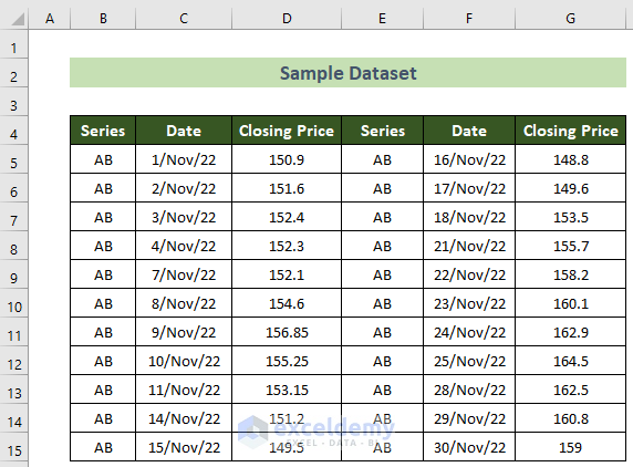
Say, you are given the closing price of a stock from the AB series for November month. You have the closing price for every weekday. Now, you want to calculate the annualized volatility of this stock. Follow the step-by-step guidelines to accomplish this.
📌 Step 1: Calculate Daily Return to Measure Annualized Volatility
The first thing you will have to do is to calculate daily returns from the given dataset.
- To do this, first, click on cell E6 and insert the following formula.
=D6/D5-1
- Subsequently, press the Enter key.

- Afterward, for all the other weekdays of the month given below, place your cursor in the bottom right position of cell E6.
- Following, drag the black Fill Handle below upon its appearance.
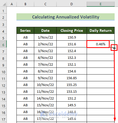
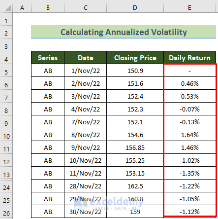
- As a result, you will see you will get all the daily returns of November month for the following stock.
Read More: How to Calculate Historical Volatility in Excel
📌 Step 2: Calculate Daily Volatility
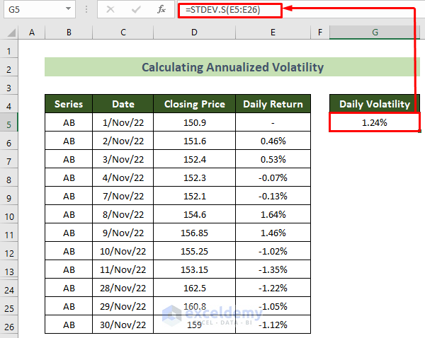
Now, you will need to calculate the Daily Volatility from the standard deviation of daily returns. You can do this by using the STDEV.S function.
- In order to calculate the daily volatility, click on cell G5 and insert the formula below.
=STDEV.S(E5:E26)
- Subsequently, hit the Enter key.
Read More: How to Calculate Realized Volatility in Excel
📌 Step 3: Calculate the Annualized Volatility
Last but not least, now you will need to calculate the annualized volatility.
- For doing this, click on cell G8.
- Following, write the formula below involving the SQRT function in the formula bar.
=G5*SQRT(252)
- Finally, press the Enter key.
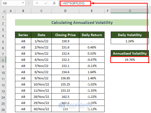
Thus, you will be able to calculate the annualized volatility successfully in Excel.
Read More: How to Calculate Implied Volatility in Excel
Download Practice Workbook
You can download our practice workbook from here for free!
Conclusion
So, in this article, I have shown you all the quick steps to calculate annualized volatility in Excel. I suggest you read the full article carefully and practice accordingly. I hope you find this article helpful and informative. You are welcome to comment here if you have any further questions or recommendations.
Related Articles
<< Go Back to Volatility In Excel | Excel for Finance | Learn Excel
Get FREE Advanced Excel Exercises with Solutions!
