Method 1 – Using DB Function in Excel
Steps:
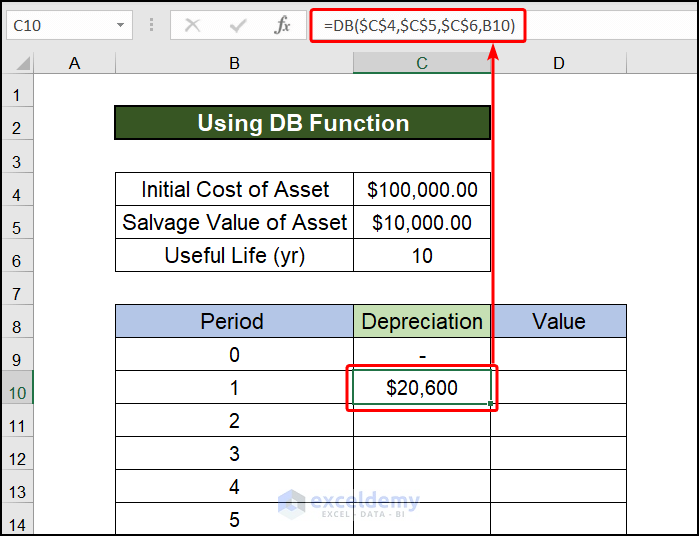
- Calculate depreciation using the Declining Balance method by entering a formula. Excel has a built-in function to make things easier for us. The name of the function is similar to the method name, DB function.
- Insert the following formula in cell C9
=DB($C$4,$C$5,$C$6,B10)$C$4= Initial Cost
$C$5= Salvage Value
$C$6= Useful Life (yr)
B10= Period
The DB function performs the following calculations.
- Fixed-rate in DB method = 1 – ((salvage Value/Initial cost) ^ (1 / life))
- Fixed rate= 1 – (10000/10,0000)^(1/10) = 1 – 0.7943282347 = 0.206
- Depreciation value period 1 = 100,000 * 0.206 =20,600
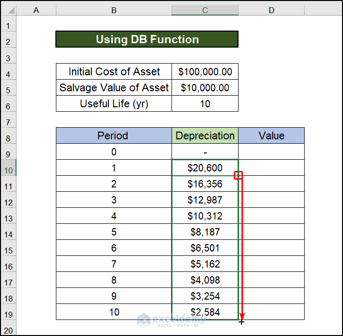
- Depreciation value period 2 = (10,000 – 2,060.00) * 0.206 = 16356
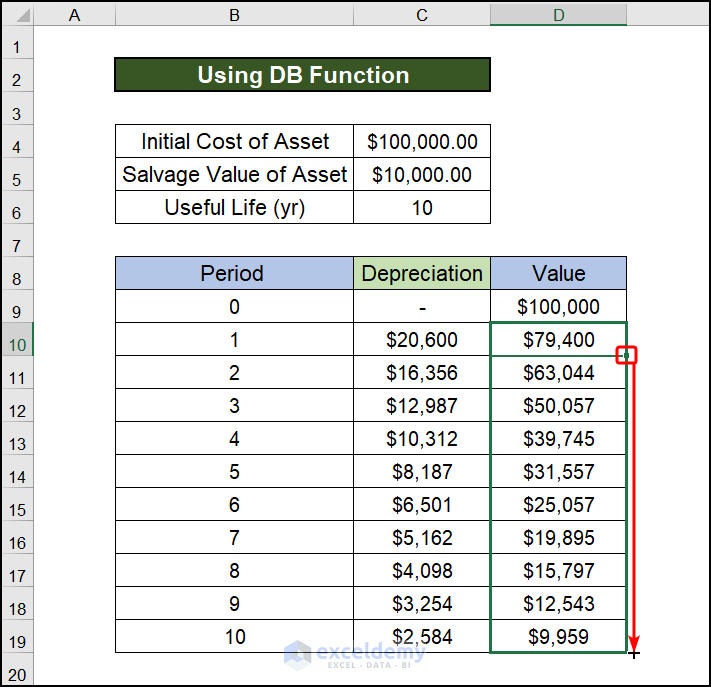
- Drag the fill handle downwards to calculate depreciation in different periods of the year. As in the following image we have calculated depreciation for the first year, the second year the tenth year.
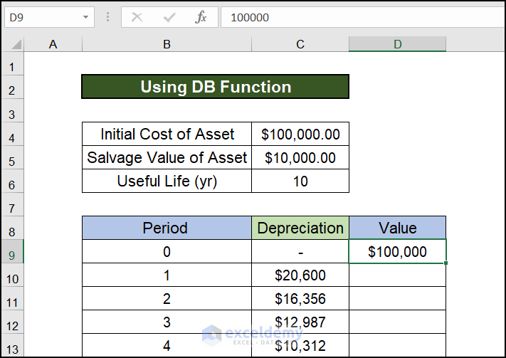
- For Period 0, we have no depreciation. The value of a particular product will be the same as the Initial Cost. We entered the Initial Cost in the cell of D9.
- As we have calculated depreciation for Period 1, we will subtract depreciation from the Initial value. After subtracting, the value of the product will be 79,400, and the simple subtraction formula will be the following:
=D9-C10D9= Initial Cost
C10= Depreciation
D9-C10= Asset Value in Period 1
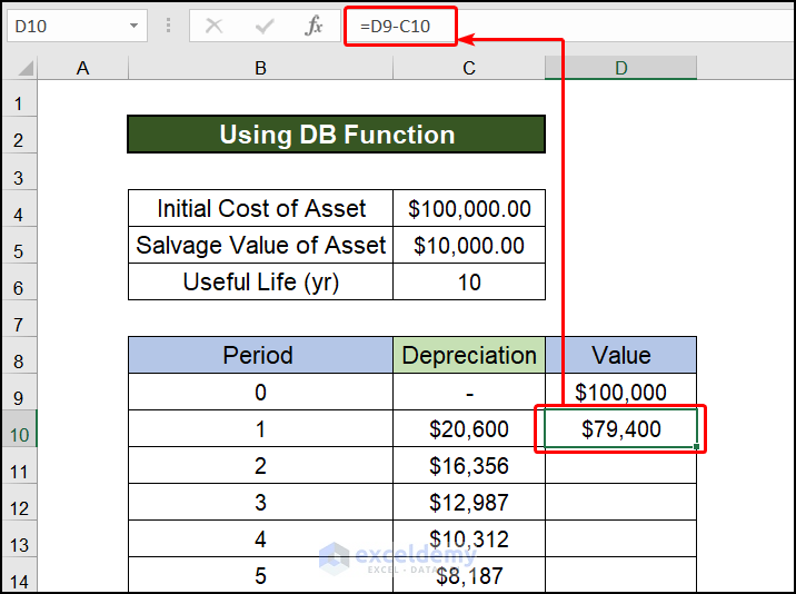
- Now, if we drag down the fill handle, as in the image below, we will get the asset value for the rest of the cells.
Method 2 – Applying DDB Function (Double Declining Balance Depreciation Formula) in Excel
Steps:
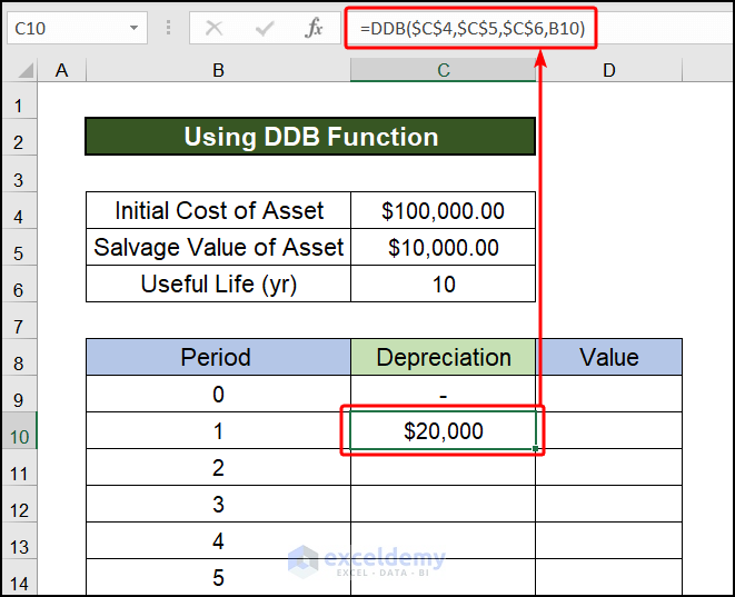
- In cell C9, we will enter the following formula to calculate depreciation:
=DDB($C$4,$C$5,$C$6,B10)$C$4= Initial Cost
$C$5= Salvage Value
$C$6= Useful Life (yr)
B10= Period
The DDB function performs the following calculations.
- Fixed-rate in DDB method = 2* (salvage Value/ Initial cost)
- Fixed rate= 2* (10000/10,0000) = 1 / 5 = 0.2
- Depreciation value period 1 = 100,000 * 0.2 =20,000
- Depreciation value period 2 = (10,0000 – 20,000) * 0.2 = 16,000.
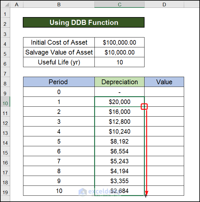
- After entering a formula, our current task is to drag the fill handle downwards to copy the formula for the rest of the periods.
- We will have depreciation in each corresponding year.
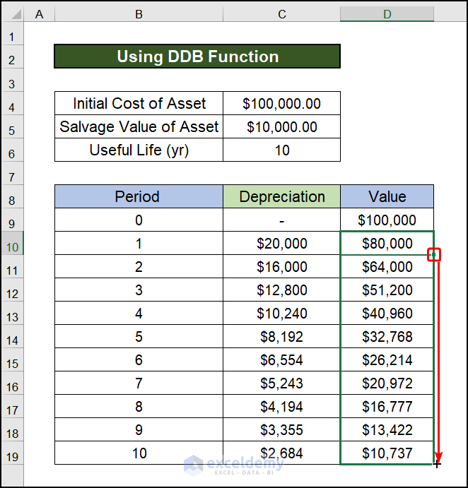
- Subtract depreciation from the Initial value, as we have calculated depreciation for Period 1. After subtracting, the value of the product will be 79,400, and the simple subtraction formula in cell D10 will be the following:
=D9-C10D9= Initial Cost
C10= Depreciation
D9-C10= Asset Value in Period 1
- Drag down the fill handle like in the figure below; we will obtain the asset value for the remaining cells.
Method 3 – Using VDB Function or Variable Declining Balance Function in Excel
Steps:
- The Calculation process of the VDB function is similar to the DDB function. But VDB turns to the straight Line method to reach salvage value.
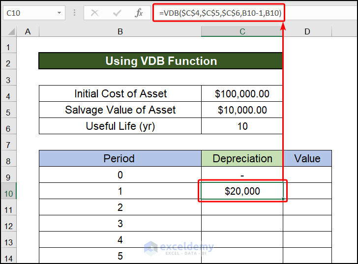
- In cell C9, we will enter the following formula to calculate depreciation:
=VDB($C$4,$C$5,$C$6,B10-1,B10)$C$4= Initial Cost
$C$5= Salvage Value
$C$6= Useful Life (yr)
B10-1= Starting Period argument will be 1-1=0
B10= Ending Period argument will be 1
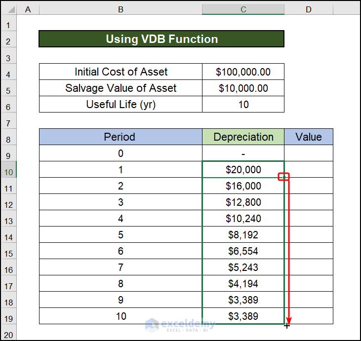
- Our current objective is to slide the fill handle downward to replicate the formula for the remaining periods after entering the formula.
- Depreciation in the corresponding year is seen in the accompanying image.
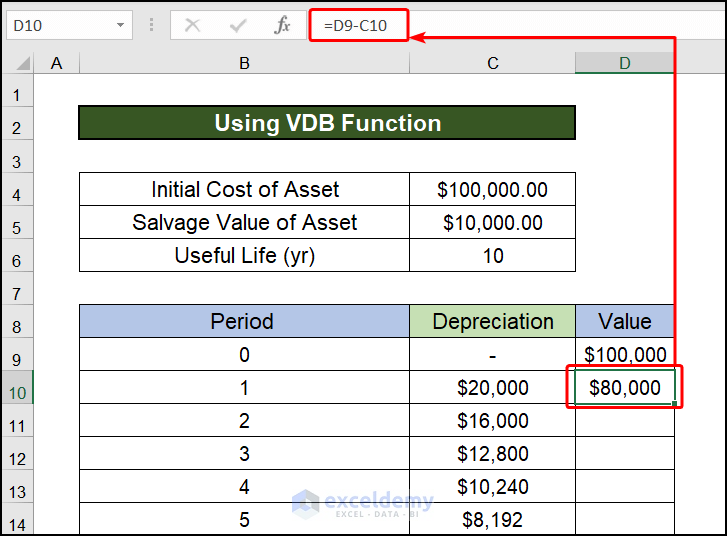
- After calculating it for Period 1, we will now deduct depreciation from the initial value. The value of the product will be 80,000 after subtraction, and the straightforward subtraction formula is as follows:
=D9-C10D9= Initial Cost
C10= Depreciation
D9-C10= Asset Value in Period 1
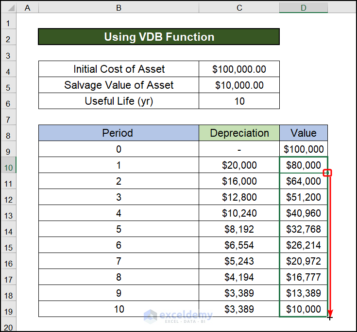
- If we drag down the fill handle like in the figure below, we will now see the asset value for the remaining cells.
Method 4 – Applying SLN Function
Steps:
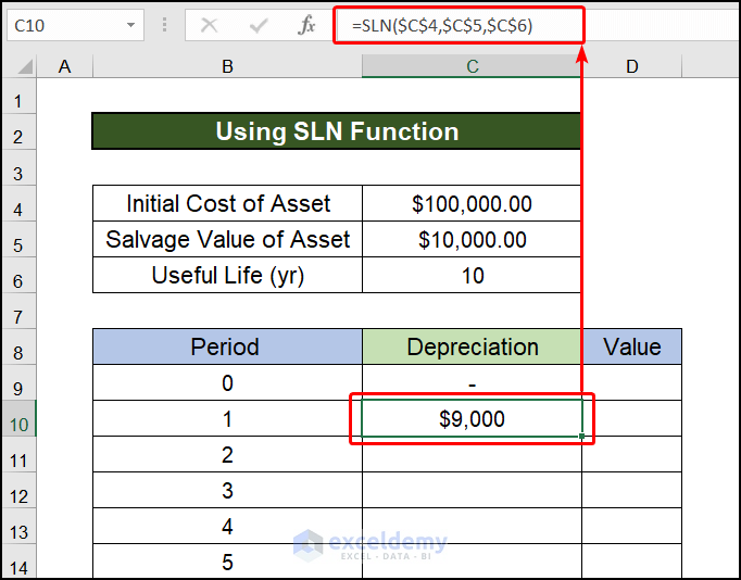
- In cell C9, we will enter the following formula to calculate depreciation:
=SLN($C$4,$C$5,$C$6)$C$4= Initial Cost
$C$5= Salvage Value
$C$6= Useful Life (yr)
B10= Period
The SLN function performs the following calculations.
- Deprecation Value = (100,000 – 10,000) / 10 = 9000.00.
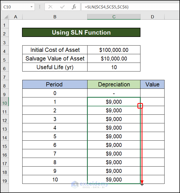
- If we subtract this value 10 times, the asset depreciates from 100,000 to 10,000 in 10 years.
- For the remaining periods after entering the formula, our current goal is to slide the fill handle lower to duplicate the formula.
- The accompanying picture shows depreciation in the relevant year.
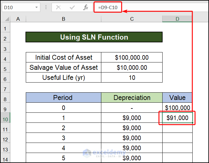
- Now that we have obtained depreciation for Period 1, we will subtract it from Initial Cost. After subtraction, the product’s value will be 91,000, and the simple subtraction formula is as follows:
=D9-C10D9= Initial Cost
C10= Depreciation
D9-C10= Asset Value in Period 1
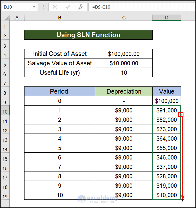
- If we drag down the fill handle, as shown in the image below, the asset value for the remaining cells will be obtained.
Method 5 – Using SYD Function
Steps:
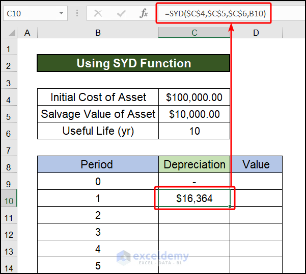
- Input the following formula to compute depreciation in cell C9.:
=SYD($C$4,$C$5,$C$6,B10)$C$4= Initial Cost
$C$5= Salvage Value
$C$6= Useful Life (yr)
B10= Period
The SYD function performs the following calculations.
- 55 years are the sum of the years 10 + 9 + 8 + 7 + 6 + 5 + 4 + 3 + 2 + 1.
- Losses Total Value = (100,000 – 10,000) = 90,000.00.
- Rate of depreciation= Remaining useful year/ sum of the years
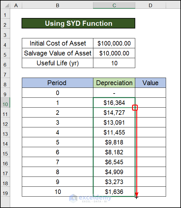
- Period 1 depreciation value = 10/55 * 90,000 = 16,364.
- Period 2 depreciation value = 9/55 * 90,000 = 14,727
- Our current goal for the remaining periods after entering the formula is to slide the fill handle lower to replicate the formula.
- The accompanying image depicts the year’s depreciation.
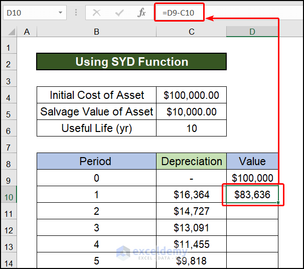
- We got the depreciation for Period 1; we will deduct it from the Initial Cost. The product’s value will be 83,636, and the simple subtraction formula is as follows:
=D9-C10D9= Initial Cost
C10= Depreciation
D9-C10= Asset Value in Period 1
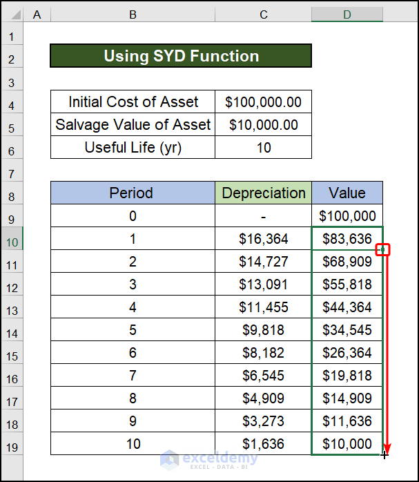
- As seen in the figure below, dragging down the fill handle will yield the asset value for the remaining cells.
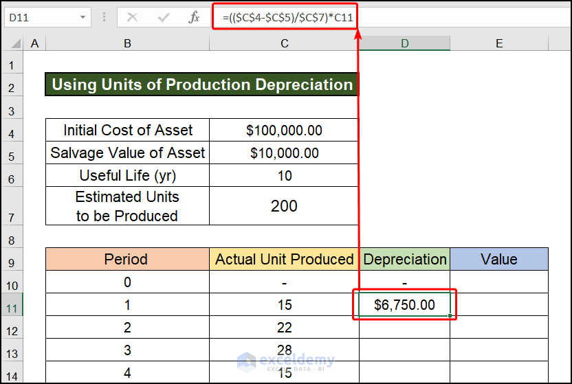
Method 6 – Applying Units of Production Formula of Depreciation for Declining Balance
Steps:
- Input the following formula to compute depreciation in cell C9:
=(($C$4-$C$5)/$C$7)*C11$C$4= Initial Cost
$C$5= Salvage Value
$C$7= Estimated Units to be Produced
C11= Actual Unit Produced
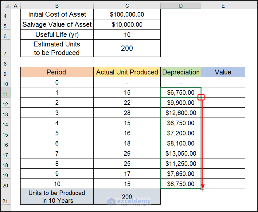
- Drag the fill handle down to complete the series.
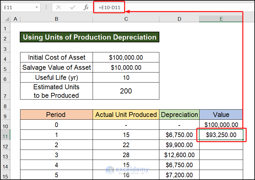
- We got a depreciation for Period 1, and we will subtract it from the Initial Cost. The product’s value will be 93,250, and the formula of subtraction is as follows:
=D9-C10D9= Initial Cost
C10= Depreciation
D9-C10= Asset Value in Period 1
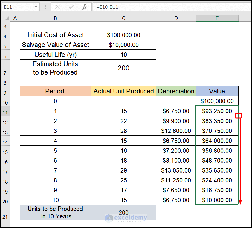
- Drag the Fill Handle downward to make the end of the calculation of depreciation using the units of production method. You get the depreciation of the declining balance by using the production method’s formula in Excel.
Some More Formulas to Calculate Declining Balance Depreciation in Excel
1. Discounted Cash Flow Formula
By discounting the anticipated future cash flows, the discounted cash flow (DCF) analysis approach is being used to value investments. In the investing sector as well as corporate financial management, DCF analysis is frequently employed since it may be used to evaluate a stock, company, or project, among many other assets or activities.
2. Insurance Policy Method
There are many commonalities between the two approaches, including the investment of depreciation as well as the replacement of equipment with the proceeds at the end of its useful lifespan. Though one significant contrast between the two approaches is: Inside the insurance policy method, services are covered for the necessary amount, and the first insurance premium is paid each year. And being under the sinking fund method, investments are made at the end of each year after the acquisition of assets. The method of an insurance policy is less dangerous since the maturity amount will undoubtedly be obtained; however, the method of a sinking fund might be riskier because the market value of the assets can fluctuate.
3. Annuity Method
The goal of the annuity method of depreciation is to achieve a steady rate of return on a property. It is most frequently applied to much more pricey capital assets with longer estimated useful lives.
4. WDV Method of Depreciation Formula
When computing depreciation, the written-down value technique, or WDV method, is a handy tool to deal the depreciation. The Diminishing Balance Method or Declining Balance Method are other names for this method. There are two approaches that are typically used to calculate depreciation.
Written Down Value (WDV), Straight Line Technique (SLM) Company policy does not put any restrictions on the use of any method. The Income-tax Act mandates that only the WDV technique be used to determine depreciation, despite the fact that Companies often utilize SLM.
When estimating assets’ net worth each year, we use this technique for a constant rate of depreciation.
Written Down Value Method = (Cost of Asset – Salvage Value of the Asset) * Rate of Depreciation (%)How to Choose a Suitable Method for a Company to Calculate Depreciation
Most public companies use the SLN method to calculate depreciation. Moreover, the depreciation of buildings and furniture is calculated through a straight-line approach.
On the other hand, the SYD, or Sum of Years’ Digits method, depreciates more in a product’s earlier lifespan than in its later period.
Usually, to calculate the depreciation of transportation, we apply the SYD or Sum of Years’ Digits method.
How to Use an Excel Template for Monthly Depreciation Calculation
Determining cumulative depreciation is simple and easy to understand using the straight-line technique. The depreciation under this technique stays constant throughout the asset’s lifetime for each succeeding year. Following are the steps to compute depreciation using this approach:
- The amount that can be depreciated is calculated by deducting the asset’s cost from its scrap value.
- Cost without the residual value equals total depreciation over the lifespan of a product.
- Now, the entire amount of depreciation needs to be divided by the asset’s lifetime in years.
- Total depreciation divided by useful lifetime equals annual depreciation.
- Lastly, after getting the value for the year using this technique, some of our Excel users may prompt to calculate the monthly depreciation, which can be obtained after dividing it by 12.
An Excel Calculator for Depreciation of Fixed Asset
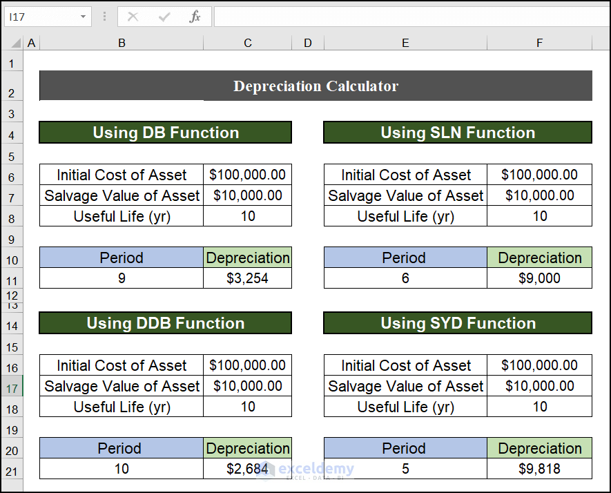
At the last moment, to make the workbook Excel user-friendly we have added a Depreciation Calculator where you can quickly calculate your depreciation of a certain product. To accomplish the process, you have to put your data for, say, Initial Cost, Useful Life, and Salvage Value in the Depreciation Calculator. Moreover, the Periodor the nth year is required to complete the calculation. A sample of a Depreciation Calculator is given in the following image.
Download Practice Workbook
You can download the practice workbook from the following download button.
Related Article
<< Go Back to Depreciation Formula In Excel|Excel Formulas for Finance|Excel for Finance|Learn Excel
Get FREE Advanced Excel Exercises with Solutions!
