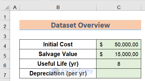
We’ll use a sample dataset, with the Initial Cost in Cell B4, the salvage Value in Cell B5, and useful life in Cell B6. We will use these cells to determine the Depreciation per yr by using the MACRS depreciation formula.
Method 1 – Using the SLN Function to Calculate MACRS Depreciation
The straight-line depreciation for one period is determined using the equation;
Straight line depreciation= (cost-salvage)/life.
Steps:
- In the C7 cell, enter the following formula.
=SLN(C4;C5;C6)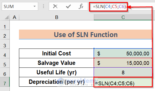
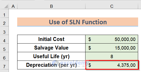
You will get the desired result.
Read More: How to Calculate Straight Line Depreciation Using Formula in Excel
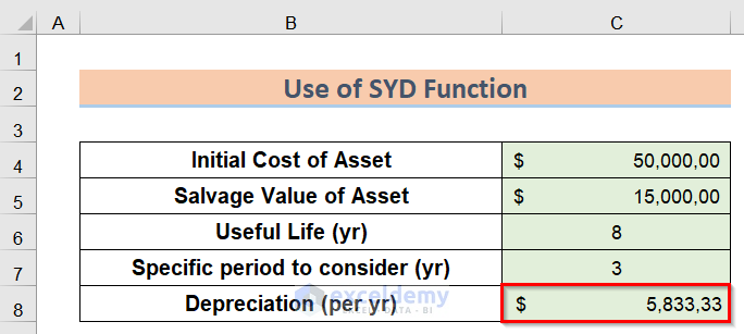
Method 2 – Using the SYD Function to Calculate MACRS Depreciation
Assets do not depreciate linearly over time. To account for this, Excel has the built-in SYD function to calculate depreciation.
Steps:
- In the C8 cell, insert the following formula.
=SYD(C4;C5;C6;C7)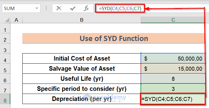
- The formula will return the output value we expected.
Method 3 – Applying the DDB Function in Excel Formula to Calculate MACRS Depreciation
A depreciation Schedule can also be prepared using the double-declining depreciation method. To apply the method, you need to use the DDB function. The function has five arguments: cost, salvage, life, period, and factor.
Steps:
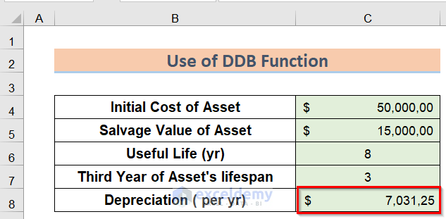
- In the C8 cell, insert the following formula.
=DDB(C4;C5;C6;C7)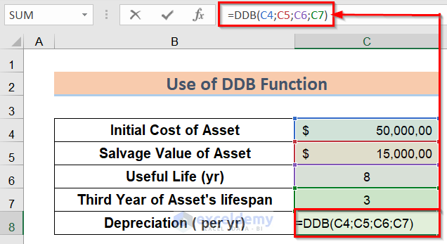
- You will get the desired result.
Read More: How to Calculate Double Declining Depreciation in Excel
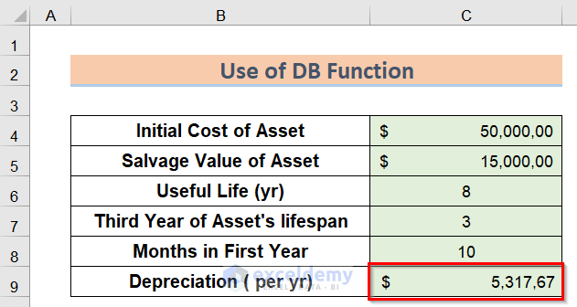
Method 4 – Using the DB Function
You can prepare a depreciation schedule using the Declining Balance depreciation method with the DB function. Cost, salvage, life, period, and month are the five inputs to the DB function. The first four arguments are mandatory, while the fifth is optional. The argument period represents the period in which the depreciation will be calculated.
Steps:
- In the C9 cell, insert the following formula.
=DB(C4;C5;C6;C7;C8)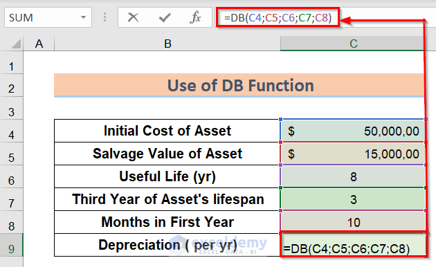
- Here’s the output.
Read More: How to Calculate Accumulated Depreciation in Excel
Method 5 – Use of the VDB Function
Since we are calculating the depreciation from a specific month span, the useful life is converted to the month. The Factor defines the rate at which the balance declines and the No_switch is used to determine the nature of the depreciation method. If the value is TRUE, Excel will not switch to a straight-line depreciation method.
Steps:
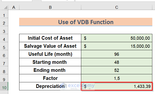
- In the C10 cell insert the following formula.
=VDB(C4;C5;C6;C7;C8;C9;TRUE)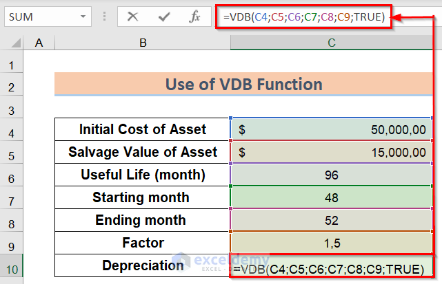
- You will get the following result.
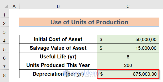
Method 6 – Using the Units of Production
The depreciation for one period using the units of production depreciation method is determined using the equation:
Depreciation=(cost-salvage)/life in units)*Units produced per period.
To use this method, you need to know the unit produced per period.
Steps:
- In the C8 cell, insert the following formula.
=((C4-C5)/C6)*C7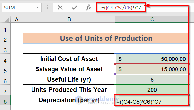
- The formula will return the output value we expected.
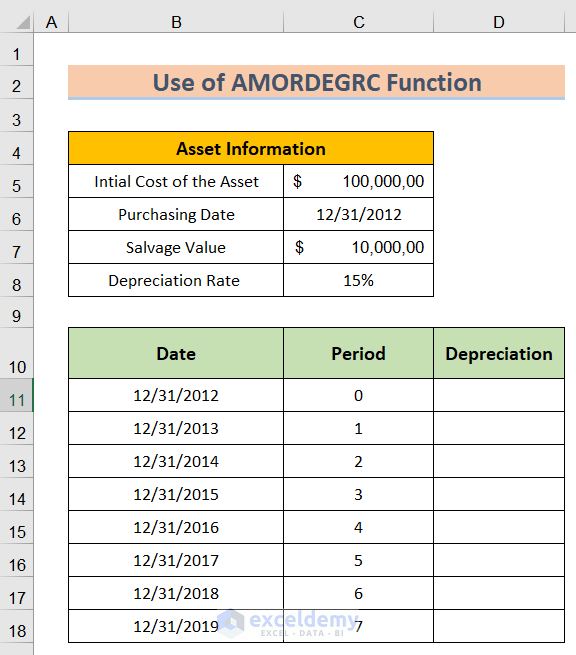
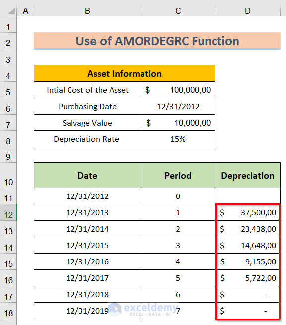
Method 7 – Utilizing the AMORDEGRC Function
The AMORDEGRC function includes a depreciation coefficient that accelerates depreciation based on the asset’s useful life.
Steps:
- Arrange a dataset like the image below.
- In the D12 cell, enter the following formula.
=AMORDEGRC($C$5;$C$6;$B$12;$C$7;C11;$C$8)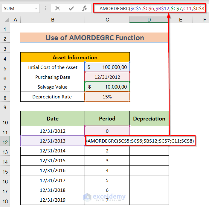
- Use the Fill Handle to apply the formula to all the desired cells.
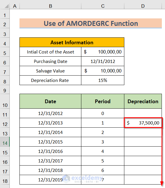
- Here’s the result.
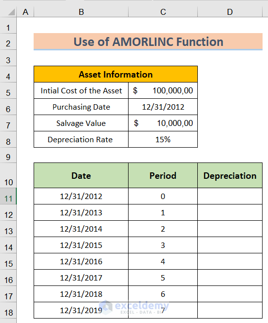
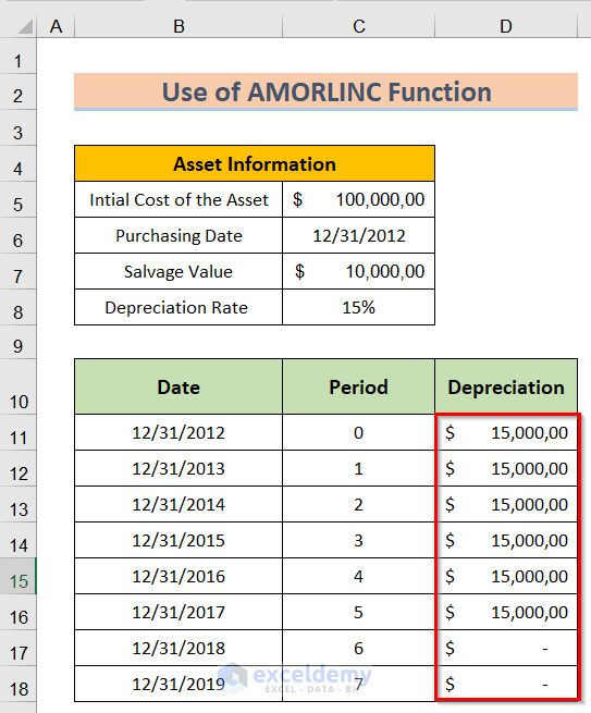
Method 8 – Applying the AMORLINC Function
his function calculates French declining balance depreciation. If you know the purchasing date of an asset, you can prepare a French straight-line depreciation schedule with a constant depreciation rate using the AMORLINC function.
Steps:
- Arrange a dataset like the image below.
- In the D11 cell, insert the following formula.
=AMORLINC($C$5;$C$6;$B$12;$C$7;C11;$C$8)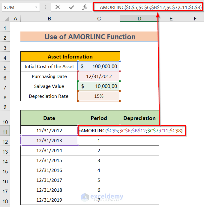
- Use the Fill Handle to apply the formula to all the desired cells.
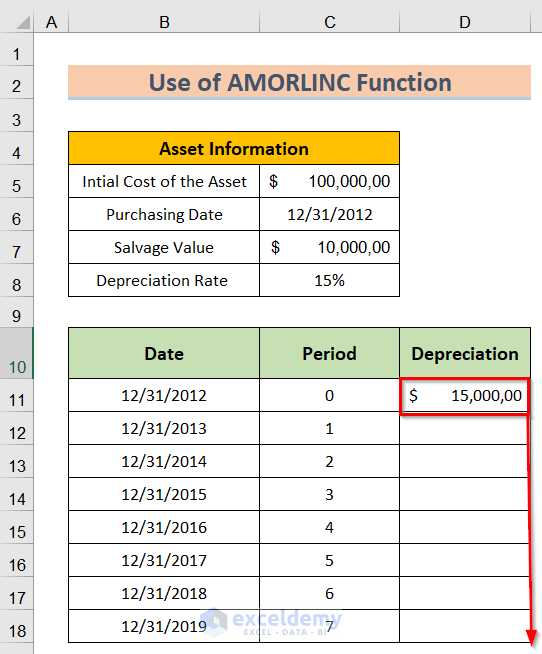
- Here’s the result.
Download the Practice Workbook
Related Articles
- How to Use WDV Method of Depreciation Formula in Excel
- How to Use Formula to Calculate Car Depreciation in Excel
<< Go Back to Depreciation Formula In Excel|Excel Formulas for Finance|Excel for Finance|Learn Excel
Get FREE Advanced Excel Exercises with Solutions!
