For a number of tasks and uses, including financial analysis to sales forecast, Excel will continue to be a crucial tool for enterprises. For instance, you can calculate your car depreciation by using an Excel workbook. So today we will learn how to use formula to calculate car depreciation in Excel.
What Is Depreciation?
Depreciation is an accounting method for distributing the cost over the course of an asset’s useful life. In financial accounting, the “Purchased Value” must be subtracted from the utility value that has been used.
Before diving into today’s topic, let’s look at the definition that is provided below for your better understanding.
- Cost of Asset: Actual cost of acquiring an asset, after taking into account all direct costs.
- Salvage Value: Salvage value is the anticipated marketable value of an item at the end of its useful life, often referred to as Residual Value.
- Useful Life of Asset: the duration of time that the asset is used. When the asset’s useful life is up, all of its value is lost.
How to Calculate Car Depreciation in Excel: 3 Methods
Let’s assume we have a dataset, namely “Car Depreciation Tally for North East Builders”. You can use any dataset suitable for you.
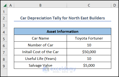
Here, we have used the Microsoft 365 version; you may use any other version according to your convenience.
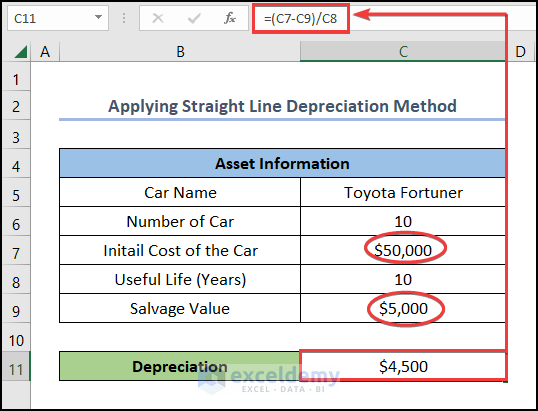
1. Applying Straight Line Depreciation Method
In straight line depreciation method, the value of the asset will be reduced over the period of useful life linearly and will end up having its salvage value.
Thus the depreciation value can be formulated as follows:
📌 Steps:
- Type the following formula in cell C11.
=(C7-C9)/C8
- Now see the output as given below.
Read More: How to Calculate Straight Line Depreciation Using Formula in Excel
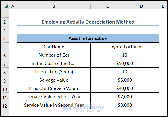
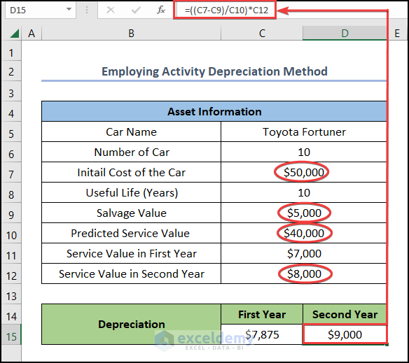
2. Employing Activity Depreciation Method
The activity depreciation method, also known as the unit of activity depreciation method, is a unique way to calculate the depreciated value of an asset, as it does not depend on its passage of time (such as years) rather than the asset’s usage.
📌 Steps:
- To calculate the cart depreciation we have chosen the following dataset as provided below.
- Now enter the following formula in the C15 cell.
=((C7-C9)/C10)*C11
Here, C7, C9, C10, and C11 refer to the Initial Cost of the Car, Salvage Value, PredictedService Value, and Service Value in First Year respectively.
- Press ENTER to see the output as given below.
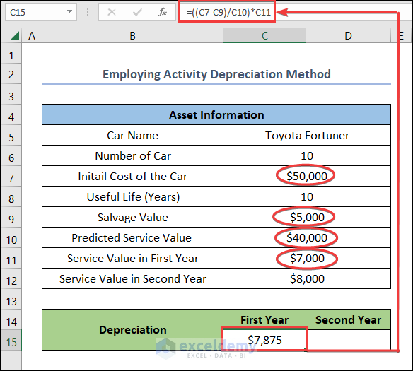
- Again enter the following formula in the D15 cell.
=((C7-C9)/C10)*C12
Here, C7, C9, C10, and C12 refer to the Initial Cost of the Car, Salvage Value, PredictedService Value, and Service Value in First Year respectively.
- Then, press ENTER to see the output.
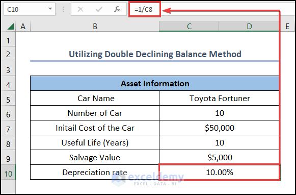
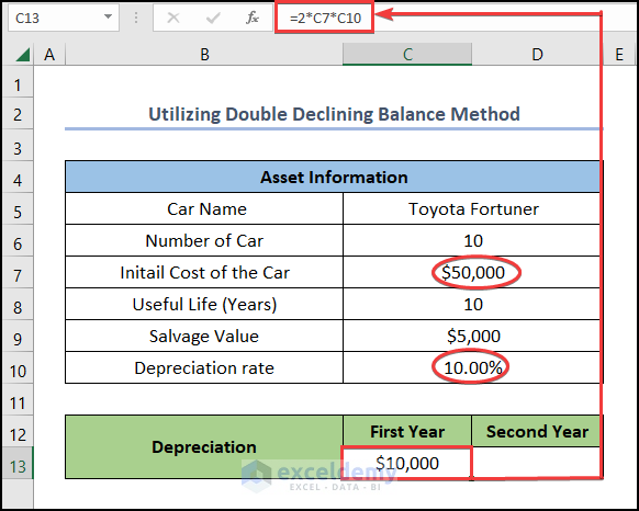
3. Utilizing Double Declining Balance Method
The double declining depreciation balance method works by multiplying the value of the straight line depreciation value twice. So now the question is why we need to use this type of method when a straight line depreciation method can do the job.
Well, the DDB depreciation method fits for those assets whose value depreciates rapidly during the first few years of their life span. Although it may also apply to company assets like electronic gadgets, mobile, cameras, etc. However, this is more usually the case for items like vehicles, motors, generators, etc.
📌 Steps:
- To begin with this method, write the following formula in cell C10.
=1/C8
- Hit ENTER to see the output.
- Now enter the following formula in cell C13.
=2*C7*C10
- Press on the ENTER button afterward.
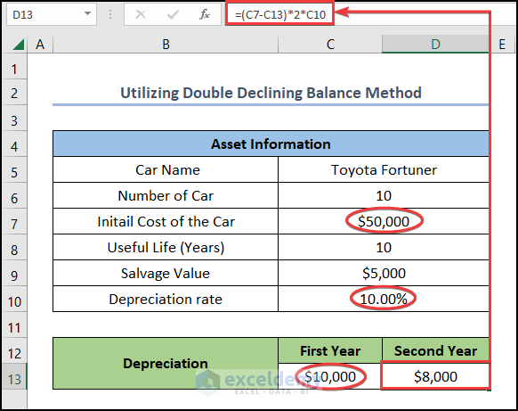
- Now do the same to cell no D13 also.
=(C7-C13)*2*C10
- See the output as given below.
Read More: How to Calculate Double Declining Depreciation in Excel
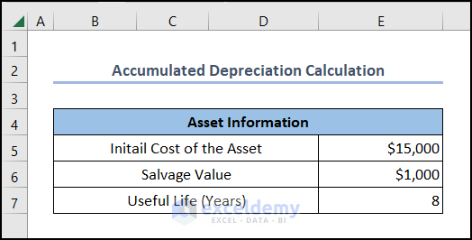
How to Calculate Accumulated Depreciation in Excel
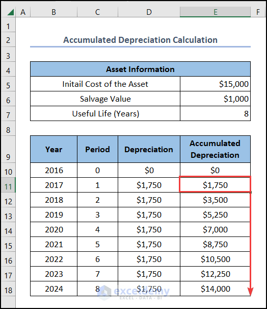
Accumulated depreciation describes the aggregated depreciation over a period of time. To begin with this method, first look at the dataset as we provided below.
📌 Steps:
- As the depreciation in the first year is zero, therefore write 0 in the D10 cell.
- Now, type the following formula in cell D11.
=($E$5-$E$6)/$E$7
Here, D5 and D6 cells represent the “Initial Cost of the Asset” and “Salvage Value” respectively.
- Press ENTER to get the output for 2017.
It is worth mentioning that here dollar sign ($) also known as absolute reference is used to lock the E5, E6 and E7 cells as those cell values will be required to calculate the value for years 2018 to 2024 as well. If you want to make this process more shortcut, press the F4 key after selecting the cell.
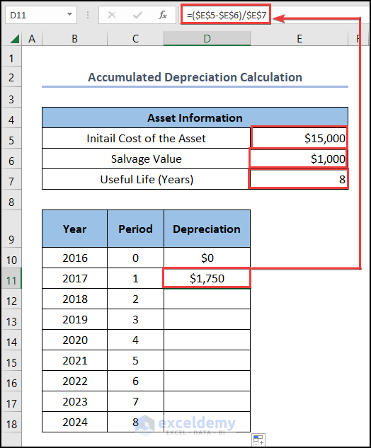
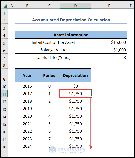
- To get the other values, drag the Fill Handle tool from D11 to D18.
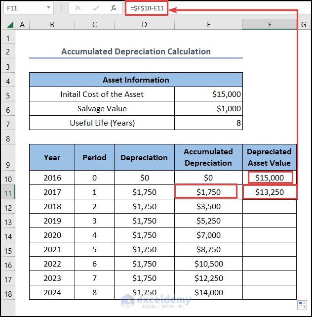
- Now to calculate accumulated depreciation, first thing first, type 0 as the initiator in the E10 cell.
- Enter the following formula in cell E11.
=E10+D11
- Then, hit the ENTER button afterward.
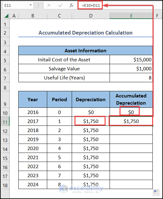
- Now drag down the Fill Handle tool to get the other value.
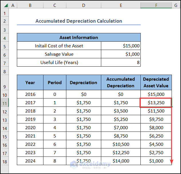
- The last step of this method is to calculate Depreciated Asset Value. First of all, enter $15,000 in the F10 cell as the initial asset value is $15,000.
- Then, simply enter the following formula in cell F11.
=$F$10-E11
Here F10 and E11 cells stand for “Depreciated Asset Value” and “Accumulated Depreciation” respectively.
- Press the ENTER button to see the result.
- Drag down the Fill Handle tool from F11 to F18 to get the other output.
Read More: Calculate Sum of Years Digits Depreciation with Formula in Excel
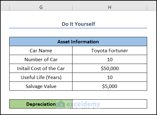
Practice Section
To practice those formulas to calculate car depreciation in Excel, We have provided a Practice section on the right side of each sheet. Please make sure to do it yourself.
Download Practice Workbook
You can download and practice the dataset that we have used to prepare this article.
Conclusion
In this article, we have discussed how to use formula to calculate car depreciation in Excel. As you have already understood, there are plenty of ways to do this task. So before going through a specific method, ensure the method you choose aligns with your work. Further, If you have any queries, feel free to comment below and we will get back to you soon.
Related Articles
- How to Use WDV Method of Depreciation Formula in Excel
- Units of Production Depreciation Method with Formula in Excel
- How to Use MACRS Depreciation Formula in Excel
- How to Apply Declining Balance Depreciation Formula in Excel
<< Go Back to Depreciation Formula In Excel|Excel Formulas for Finance|Excel for Finance|Learn Excel
Get FREE Advanced Excel Exercises with Solutions!
