Depreciation is a very common term in the case of assets. In general, it is the decline of an asset over a certain period of time. There are many methods to calculate any asset’s depreciation. In this article, we will calculate the sum of years’ digits depreciation with formula in Excel. Microsoft Excel has introduced some wonderful techniques and formulas to calculate this. Therefore, we will learn to calculate the sum of years’ digits depreciation with formula in Excel using 2 easy methods.
What Is Sum of Years Digits Depreciation?
The sum of years’ digits is one of the methods to calculate the depreciation of an asset. It is used to find the useful life of an asset in the first few years. It is also called the SYD method.
The SYD method gives a more accurate result than any other method of calculating depreciation. It is because the SYD method considers a larger amount of production capacity comparing earlier years and later days. The chosen method of depreciation only differentiates based on the timing of recognition.
The SYD method has an impact on cash flows, taxable income and income tax payments into later periods of time.
Sum of Years Digits Depreciation Formula
The Sum of years’ digits depreciation can be calculated with two methods- simple mathematical formula and an Excel formula. Both formulas are based on four arguments. They are:
- Cost: The primary cost of an asset.
- Salvage: The value of the asset when the depreciation ends after a certain period. This value can be Zero (0) as well.
- Life: It is the availability of the asset measured as a period of time through which the asset’s value will depreciate.
- Per: The period of time for calculation.
Now, let us see both of the formulas based on these arguments.
SYD=((cost-salvage)*(life-per+1)*2)/(life*(life+1))
=SYD(cost,salvage,life,per)
Calculate Sum of Years Digits Depreciation with Formula in Excel: 2 Easy Methods
As we know the formulas of the sum of years’ digits depreciation, let us follow the methods below to calculate it.
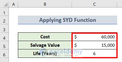
1. Apply SYD Function to Calculate Sum of Years Digits Depreciation
In this first method, we will apply the SYD function for the calculation sum of years’ digits depreciation. Let’s see how it works.
- First, insert the values of Cost, Salvage Value and Life in the Cell range C4:C6.
- Then, insert the number of years in the Cell range B9:B14 titled as Period. It defined the length of time to calculate individual depreciation.

- Now, select Cell C9 and insert this formula.
=SYD($C$4,$C$5,$C$6,B9)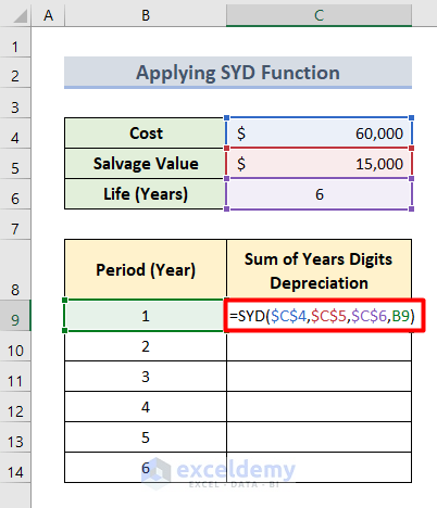
- In the following step, hit Enter and you will get the depreciation value for the first year.

- Afterward, apply the AutoFill tool and you will get all the depreciation values for each year.

- Lastly, apply this formula in Cell C15.
=SUM(C9:C14)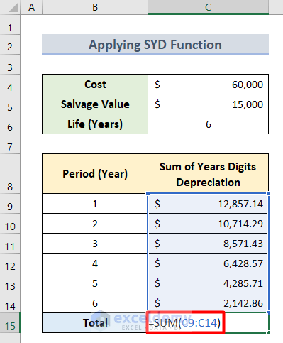
- Finally, press Enter and you will see the sum of years’ digits depreciation value.

Here, the SUM function calculates the total number of depreciation in the Cell range C9:C14.
Read More: How to Apply Declining Balance Depreciation Formula in Excel
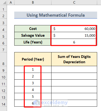
2. Find Sum of Years Digits Depreciation with Mathematical Formula
Another efficient way is to use the mathematical formula that we showed earlier in this article. With this formula, we can calculate the sum of years’ digits depreciation following the steps below.
- In the beginning, insert the same values of Cost, Salvage and Life that we used in the first method.
- Along with it, we are considering a similar time period in the Cell range B9:B14.
- Now, select Cell C9 and type this formula in it.
=(($C$4-$C$5)*($C$6-B9+1)*2)/($C$6*($C$6+1))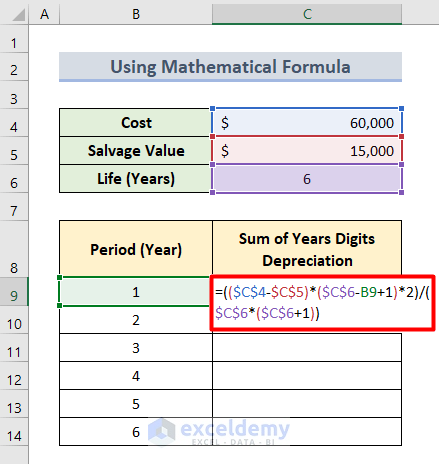
- Then, press Enter to get the first value of depreciation.

- After this, drag the Fill Handle down up to Cell C14 to get all the values for each period.

- Lastly, use this formula in Cell C15 to get the sum of years’ digits depreciation.
=SUM(C9:C14)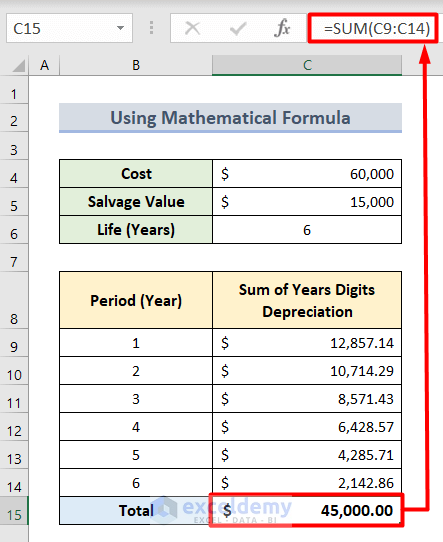
Read More: How to Calculate Straight Line Depreciation Using Formula in Excel
Things to Remember
- The unit of Life and Per will always have to same, such as days, months, or years.
- Make sure to avoid any non-numeric values, otherwise, it will show #VALUE! error.
- If Salvage or Per values are equal or less than Zero (0), it will result in #NUM! error.
- When Life < Per, then it also causes #NUM! error.
Download Practice Workbook
Download this sample workbook to practice applying your required values.
Conclusion
Henceforth, that is all for today’s article. I hope you will find the 2 easy methods useful to calculate the sum of years’ digits depreciation with formulas in Excel. Let us know your insightful suggestions in the comment box.
Related Articles
- How to Use WDV Method of Depreciation Formula in Excel
- Units of Production Depreciation Method with Formula in Excel
- How to Use SLM Method of Depreciation Formula in Excel
- How to Use MACRS Depreciation Formula in Excel
- How to Calculate Accumulated Depreciation in Excel
- How to Use Formula to Calculate Car Depreciation in Excel
- How to Calculate Double Declining Depreciation in Excel
<< Go Back to Depreciation Formula In Excel|Excel Formulas for Finance|Excel for Finance|Learn Excel
Get FREE Advanced Excel Exercises with Solutions!
