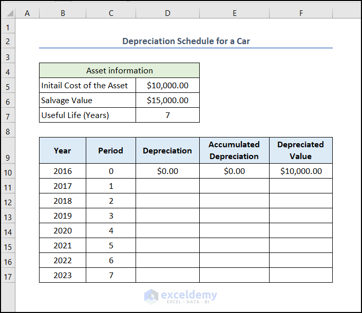
This is the sample dataset: “Depreciation Schedule for a Car”.
Method 1- Using an Arithmetic Formula
Steps:
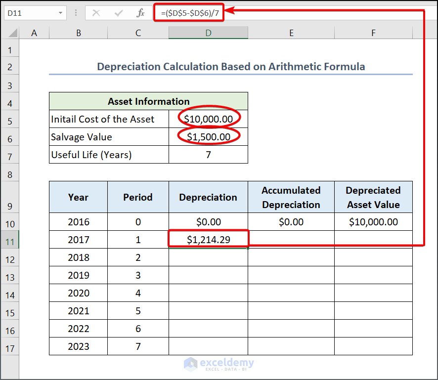
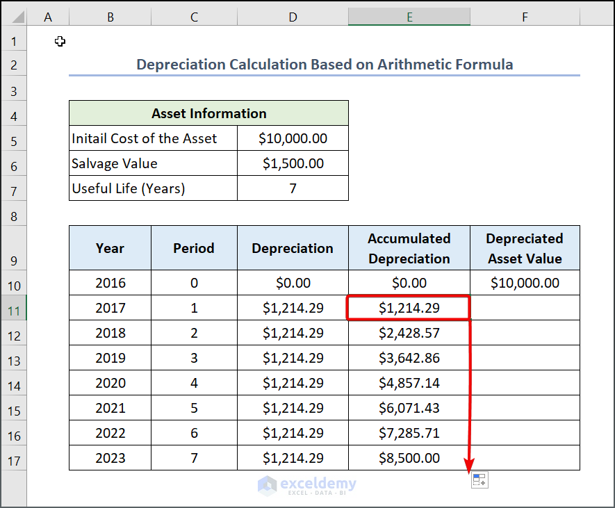
- Enter the following formula in D11.
=($D$5-$D$6)/7Here, D5 and D6 represent the “Initial Cost of the Asset” and “Salvage Value”.
As the useful life is 7 years, the subtracted value is divided by 7.
- Press ENTER to get the straight line depreciation value for 2017.
The dollar sign ($) is used to lock D5 and D6, as these values will be used to calculate the value for 2018 to 2023. You can also create an absolute reference pressing F4 after selecting a cell.
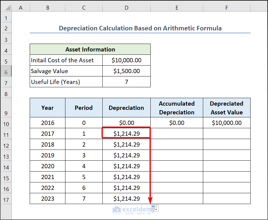
- Drag down the Fill Handle to see the result in the rest of the cells.
- To calculate the Accumulated Depreciation, enter the following formula in E11.
=E10+D11- Press ENTER.
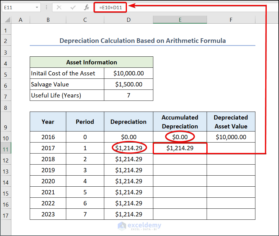
- Drag down the Fill Handle to see the result in the rest of the cells.
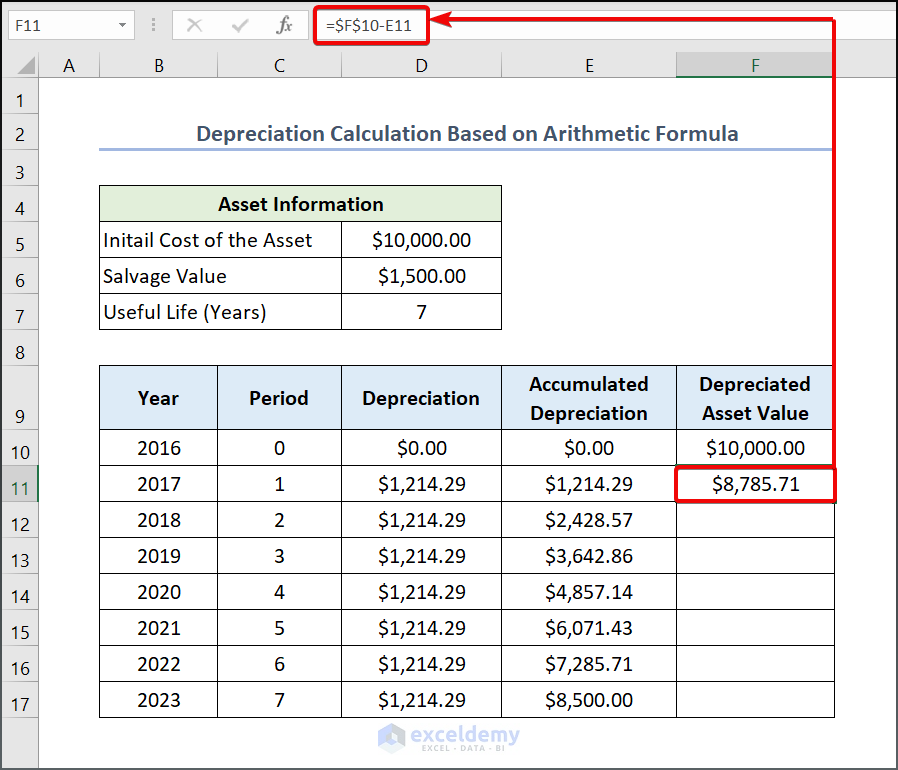
- Calculate the Depreciated Asset Value: enter the following formula in F11.
=$F$10-E11Here F10 and E11 stand for “Depreciated Asset Value” and “Accumulated Depreciation”.
- Press ENTER.
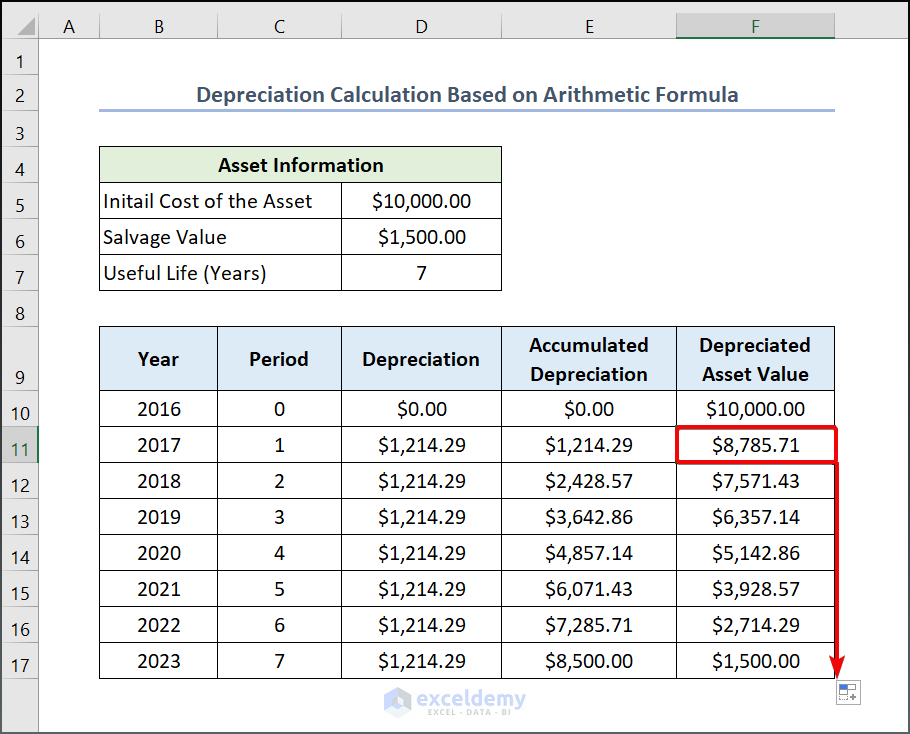
- Drag down the Fill Handle to see the result in the rest of the cells.
Read More: How to Use Formula to Calculate Car Depreciation in Excel
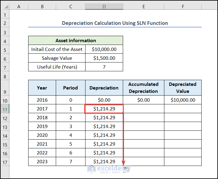
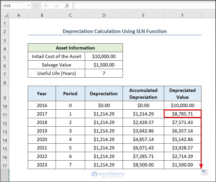
Method 2 – Using the SLN Function
Steps:
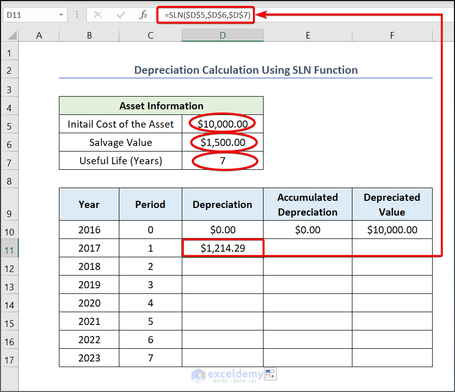
- Call the SLN function by entering an Equal sign (=) and the function.
- Enter the initial cost of asset, salvage value, and useful life in D5, D6, and D7.
- Press ENTER.
- Drag down the Fill Handle to see the result in the rest of the cells.
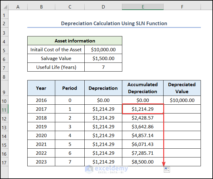
- To calculate the Accumulated Depreciation, enter the following formula in E11
=E10+D11- Press ENTER.
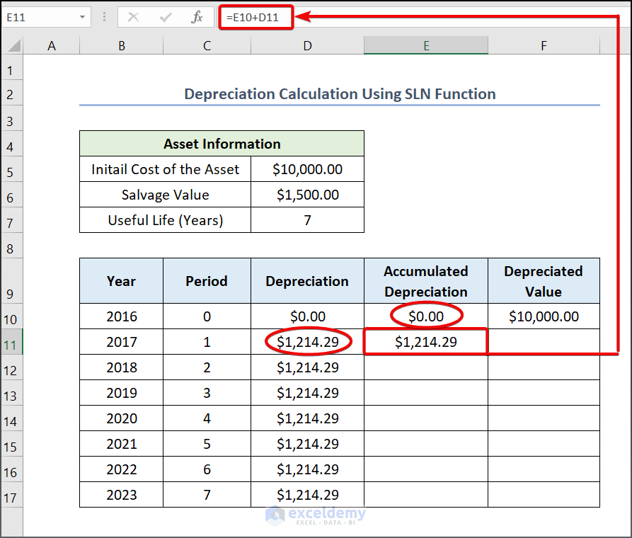
- Drag down the Fill Handle to see the result in the rest of the cells.
- To calculate the Depreciated Value, enter the formula:
=$F$10-E11- Press ENTER.
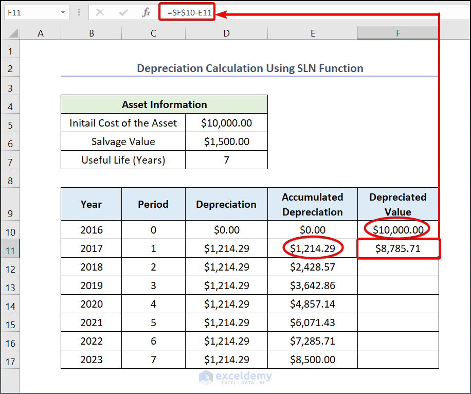
- Drag down the Fill Handle to see the result in the rest of the cells.
Method 3 – Calculating the Straight Line Depreciation for Multiple Investments
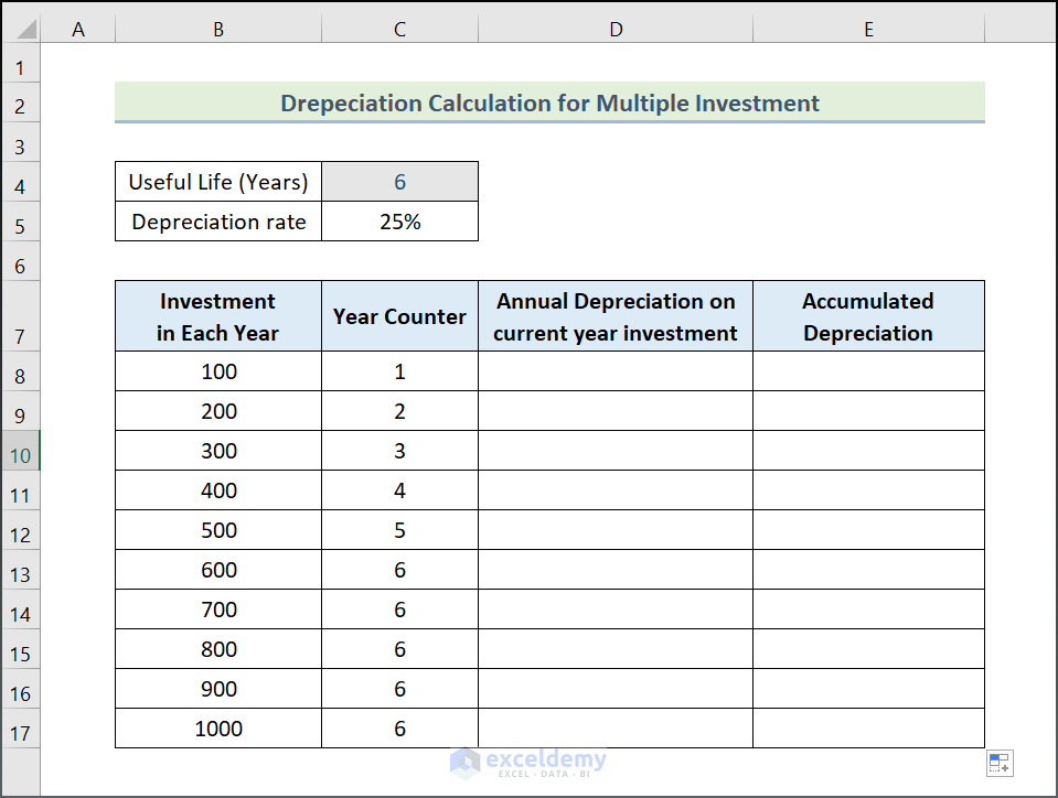
Steps:
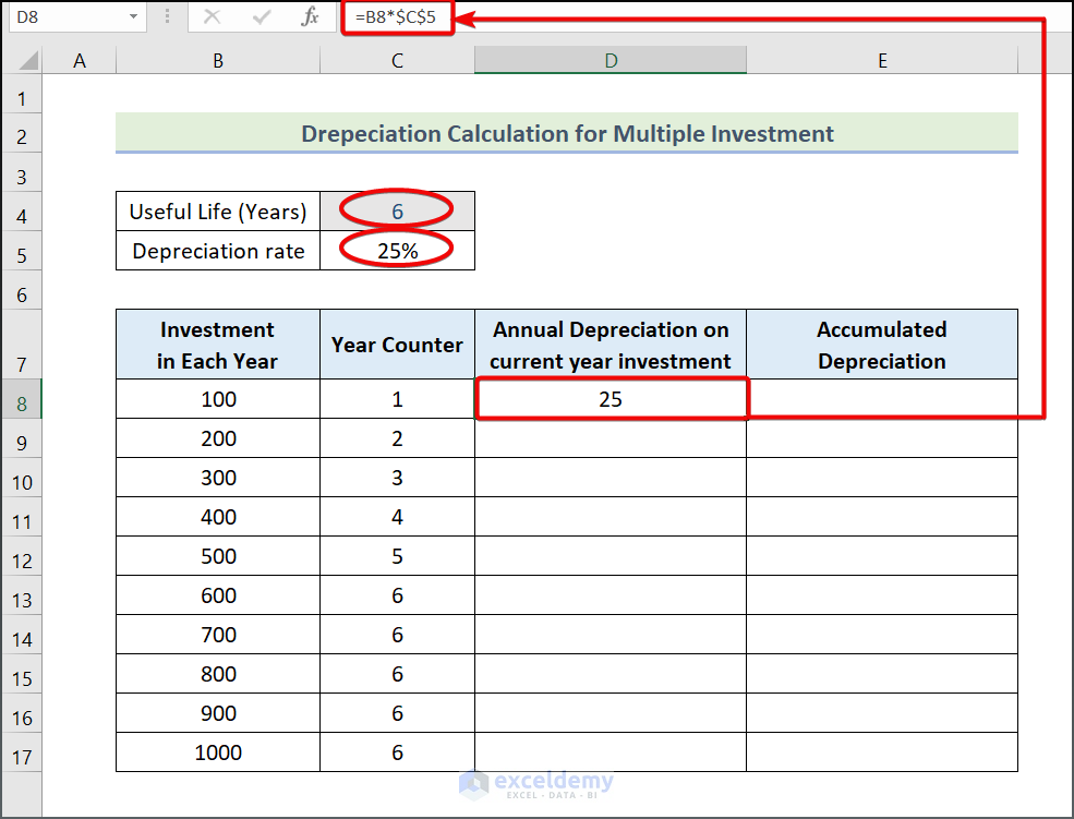
- Enter the following formula in D8.
=B8*$C$5- Press ENTER.
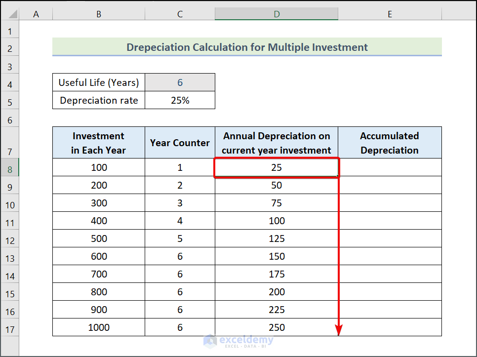
- Drag down the Fill Handle to see the result in the rest of the cells.
To calculate the accumulated depreciation for multiple investments in each year, use the OFFSET function to sum the annual depreciation in the last 6 years.
- Enter the following function:
=SUM(OFFSET(D8,,,-C8))The arguments used are: reference, rows, columns, height, and width. The first three arguments are required, the other two are optional. However, to sum the numbers in the Year Counter column, the rows, columns, and height arguments are skipped by entering the comma symbol (,). A negative sign is assigned to C8. The negative notation adds the reference cell to the number of cells above.
Note: The width argument was used to calculate the sum vertically. To do it horizontally, input the height argument.
- Press ENTER.
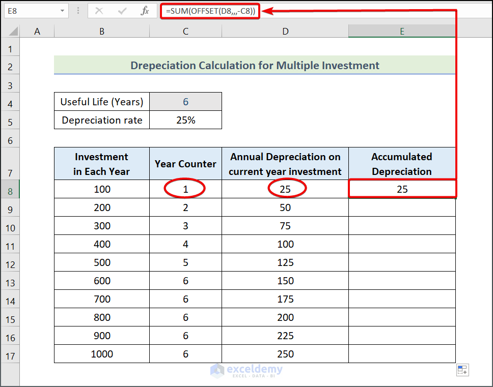
- Drag down the Fill Handle to see the result in the rest of the cells.
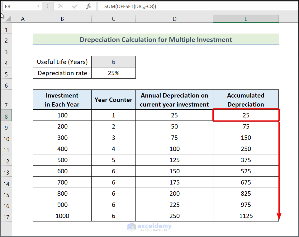
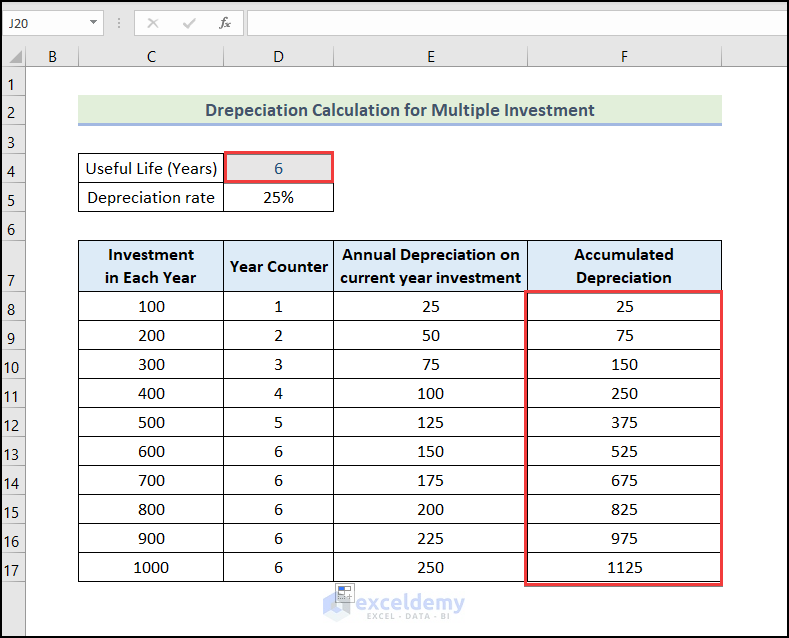
This is the output.
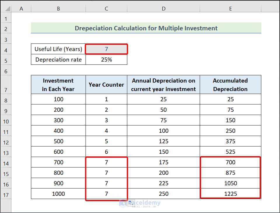
- If you count 7 years instead of 6, the Year Counter and its corresponding Accumulated Depreciation values will be the following:
Read More: Calculate Sum of Years Digits Depreciation with Formula in Excel
Practice Section
Practice here.
Download Practice Workbook
Download and practice.
Related Articles
- How to Use WDV Method of Depreciation Formula in Excel
- How to Apply Declining Balance Depreciation Formula in Excel
- Units of Production Depreciation Method with Formula in Excel
- How to Use MACRS Depreciation Formula in Excel
- How to Calculate Double Declining Depreciation in Excel
<< Go Back to Depreciation Formula In Excel|Excel Formulas for Finance|Excel for Finance|Learn Excel
Get FREE Advanced Excel Exercises with Solutions!
