How to Add Error Bars in Excel (3 Suitable Ways)

Using error bars is one of those frequent tasks that we do to describe a dataset precisely. If you are finding ways of how to add error bars in Excel, this is the right place for you. Here, in this article, you will find step-by-step ways to add error bars in Excel.

Download Practice Workbook

What Is an Error Bar?

Error Bar is a graphical representation. It describes the variability of data and represents the error or uncertainty in a given data. It can give a general idea about the data.

3 Ways to Add Error Bars in Excel

1. Using Chart Elements to Add Error Bars in Excel

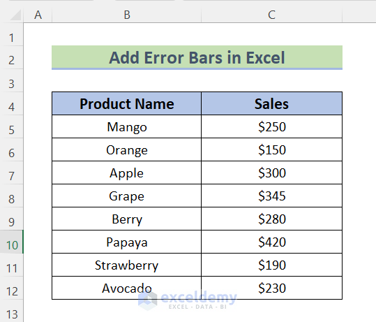
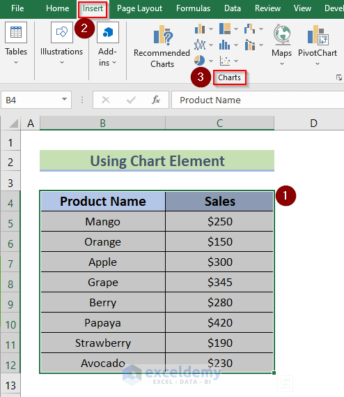
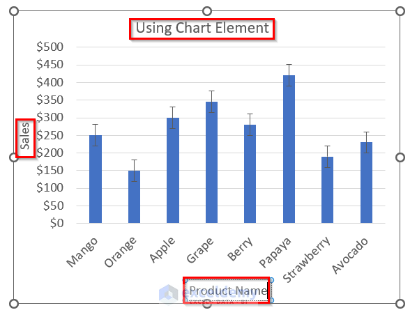
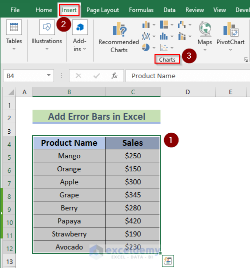
Here, we have the following dataset containing the list of Fruits and their amount of Sales. First, we will see the graphical representation of the data in the Bar charts. Then, we will show you how to add the error bars in excel.

Error bars can be added to the graph from chart elements. You can find step-by-step ways to add error bars in Excel below.

Steps:

• First, select the data from Cell B4:C12.
• Then, go to Insert >> Chart.

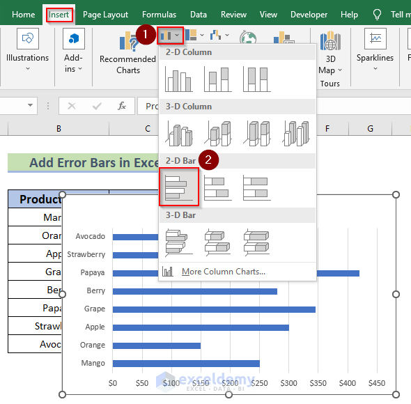
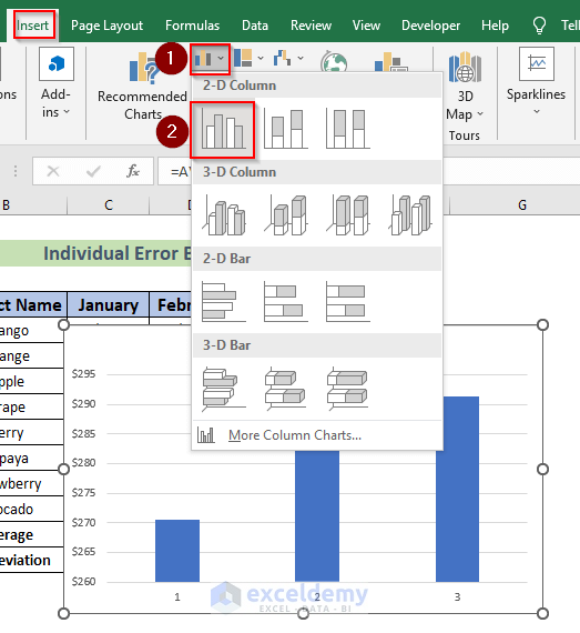
• After that, from the Bar charts select the 2-D column.

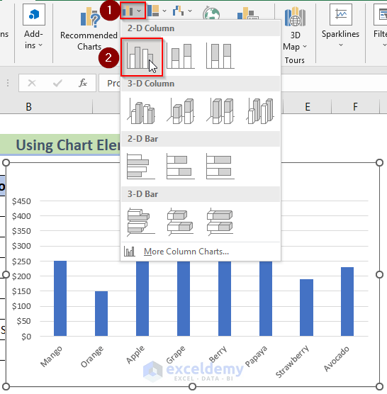
• Finally, a Bar chart is created containing the values of the dataset.

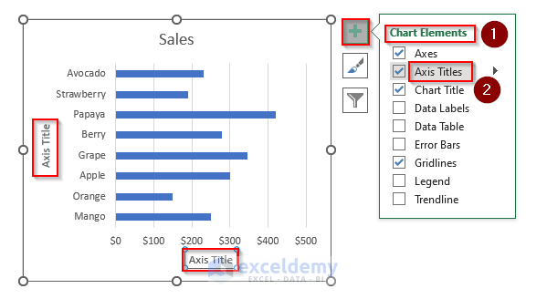
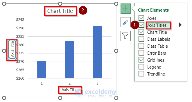
• Now, click on the ‘+’ You will be able to see the Chart Elements.
• Then, add Axis Titles and Error Bars from there.

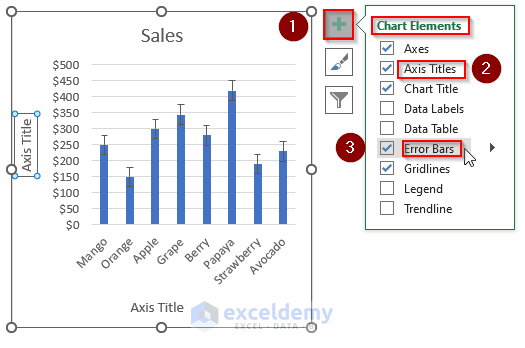
• Finally, Error Bars are added to the Bar chart using Chart Elements.

1.1. Inserting Standard Error Bars

In statistics, Standard error is a mathematical technique for calculating variability. It allows one to evaluate the standard deviation of a given sample. It is expressed as SE which is used to calculate a sample’s efficiency, accuracy, and consistency.

To add the Standard Error bar in the Bar chart you have to follow the following steps.

Steps:

• First, select the Bar chart and click on the ‘+’ sign.
• Then, from Chart Elements select Error Bars >> then select Standard Error.
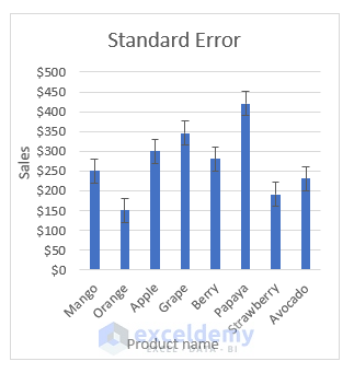
• Finally, you can see the Standard Error Bars in the chart.

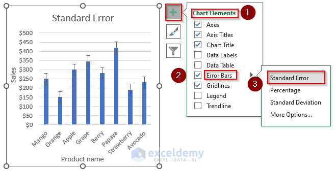
• The resultant chart shows Standard Error Bars.

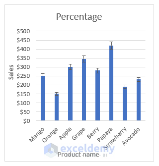
1.2. Using Percentage Error Bars

Percentage Error bar shows the fluctuation of each data point in a dataset in percentage.
To add the Percentage Error bar in the Bar chart you have to follow the following steps.

Steps:

• First, select the bar chart and click on the ‘+’ sign.
• Then, from Chart Elements select Error Bars >> Percentage Error.
• Finally, you can see the Percentage Error Bars in the chart.

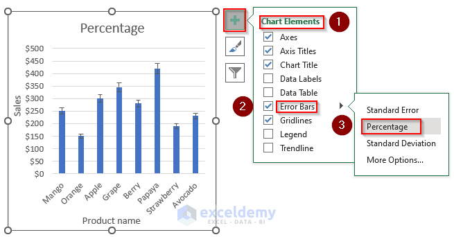
• The resultant chart shows Percentage Error Bars.

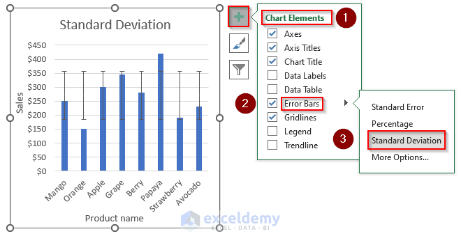
1.3. Inserting Standard Deviation Error Bars

The Standard Deviation is a measure of how evenly distributed data is. It shows how widely your data is distributed around the mean or average. Its symbol is σ.
To add the Standard Deviation Error bar in the Bar chart, you have to follow the following steps.

Steps:

• First, select the bar chart and click on the ‘+’ sign.
• Now, from Chart Elements select Error Bars >> Standard Deviation Error.
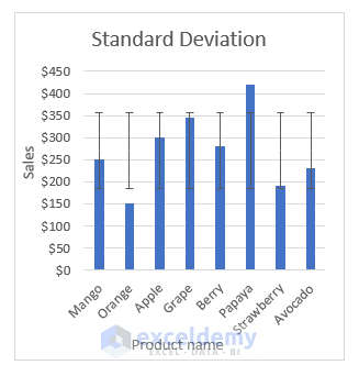
• Finally, you can see the Standard Deviation Error Bars in the chart.

• The resultant chart shows Standard Deviation Error Bars.

Read More: How to Add Custom Error Bars in Excel (2 Examples)

2. Inserting Vertical and Horizontal Error Bars in Excel

We can add both Vertical and Horizontal Error Bars to our dataset. You will find ways to add these error bars below.

2.1. Adding Vertical Error Bars

We can add Vertical Error Bars where data is represented in a Bar chart. You can find the step-by-step ways to add vertical error bars below.

Steps:

• To bring the Vertical Bar Chart follow the steps explained in Method_1.
• Next, select the chart and click on the ‘+’ sign.

• Then, from Chart Elements select Error Bars >> More Options.

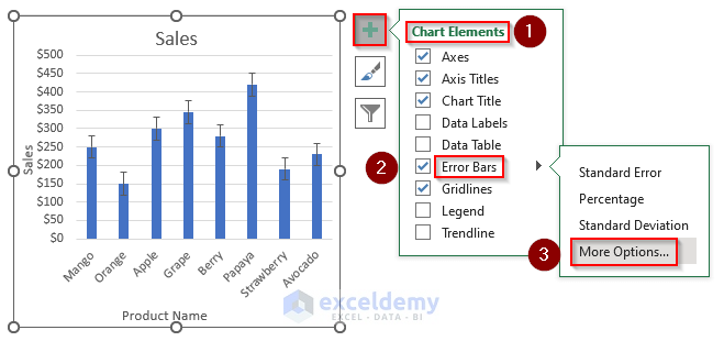
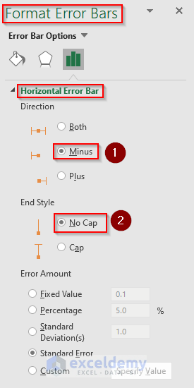
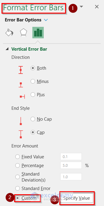
• This will open Format Error Bars.
• Then, under Vertical Error Bar, choose the options you want. Here, we choose Direction as Plus and End Style as No Cap.

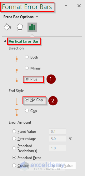
• Finally, you will get the required chart with Vertical Error Bars.

2.2. Adding Horizontal Error Bars

Horizontal error bars can be added to Bar charts, XY scatter plots and bubble charts.

Here, we will create a Bar chart using the dataset and add Horizontal Error Bars to the chart.

Steps:

• First, select the dataset from Cell B4:C12.
• Then, go to Insert >> Charts.

• After that, from Bar Charts select 2-D Bar.

• Now, select the chart and click on the ‘+’ sign.
• Chart Elements will appear.
• From there add Axis Titles.

• Now, from Chart Elements click on Error Bars >> More Options.

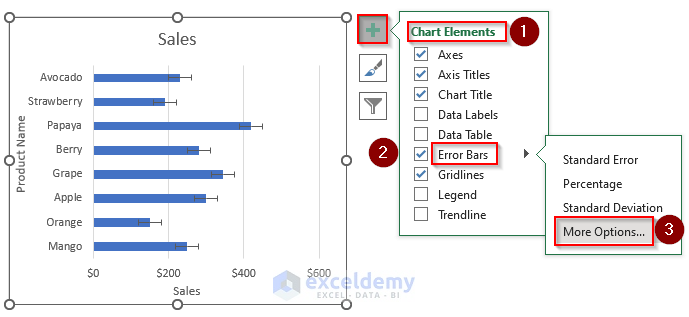
• This will open Format Error Bars.
• Finally, under Horizontal Error Bar, choose the options you want. Here, we choose Direction as Minus and End Style as No Cap.

• Finally, you will get the required chart with Horizontal Error Bars.

Read More: How to Add Vertical Error Bars in Excel (With Easy Steps)

3. Adding Individual Error Bars in Excel

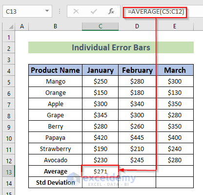
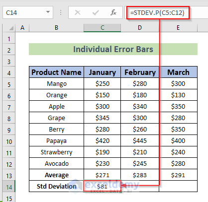
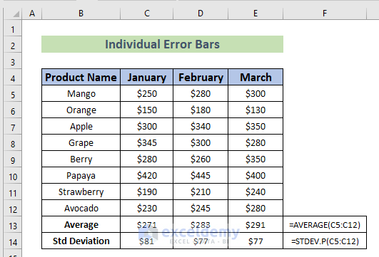
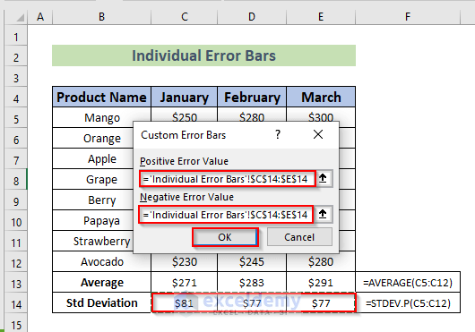
Here, we have a dataset containing the sales value of fruits for three consecutive months January, February and March. Average sales for each month are calculated using the AVERAGE function and the Standard deviation is calculated using the STDEV.P function.

Steps:

• First, select Cell C13 and insert the following formula.

• Then, press ENTER to get the Average value.

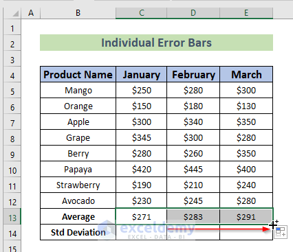
• Now, drag down the Fill Handle tool to AutoFill the formula for the rest of the cells.

• After that, select Cell C14 and insert the following formula.

• Then, press ENTER to get the Standard Deviation.

• Finally, drag down the Fill Handle tool to AutoFill the formula for the rest of the cells.

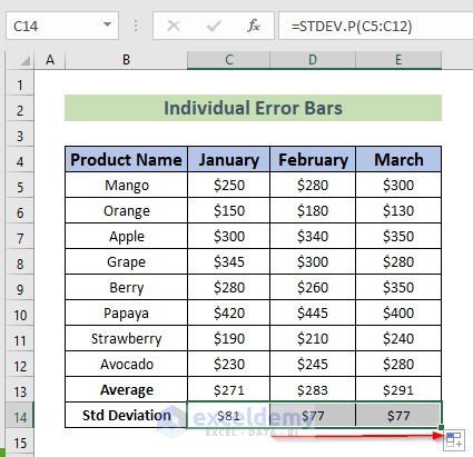
• The final dataset is given below.

Now, we will create a Bar chart using the Average value of the sales in each month. Then, we will add the Standard deviation Error bars to the chart.

Steps:

• First, select the Cells C13:E13.
• Then, go to Insert >> Charts.

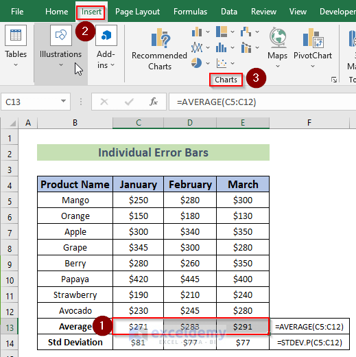
• After that, From Bar Charts >> select 2-D Column.

• Then, select the chart and click on the ‘+’ sign.
• From Chart Elements add Axis Titles and change the Chart Title.

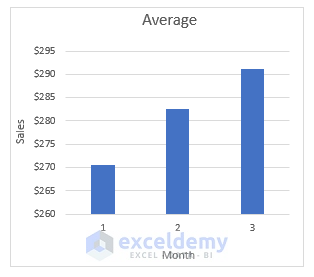
• Finally, the bar chart for the Average sales is created.

• Now, click on the ‘+’ sign.
• From Chart Elements select Error Bars >> More Options.

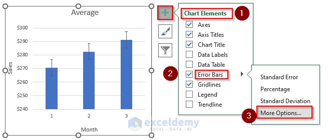
• This will open Format Error Bars.
• Then, under Vertical Error Bar, select Custom >> Specify Value.

• This will appear Custom Error Bar tool.
• Select the values from Cell C14:E14 for both Positive Error Value and Negative Error Value.
• Finally, press OK.

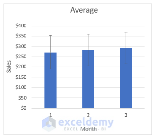
• Finally, the desired chart is prepared.

Read More: How to Add Individual Error Bars in Excel (With Easy Steps)

Conclusion

So, in this article, we have shown you how to add error bars in Excel. I hope you found this article interesting and helpful. If something seems difficult to understand, please leave a comment. Please let us know if there are any more alternatives that we may have missed. And, visit ExcelDemy for many more articles like this. Thank you!

Related Articles

• How to Remove Horizontal Error Bars in Excel (4 Quick Methods)
• How to Add Horizontal Error Bars in Excel (With Easy Steps)