A lot of times, we work with different kinds of charts in Excel. Charts or graphs help us to analyze the data more effectively. Moreover, we can also figure out the errors or how much it’s deviating from an ideal value with the help of error bars. In this article, we’ll show you the step-by-step procedures to add Vertical Error Bars in Excel.
Introduction to Error Bars in Excel
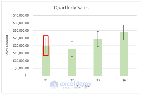
The Bars in Excel Charts that help us visualize the error margins in our dataset are known as Error Bars. It’s a very useful tool to indicate the variation or standard deviation of our data. It shows the level of accuracy in our measurement. This bar will also exhibit how much or how less our measured value is from the ideal one. We can insert the Vertical Error Bars in a bar, column, line, scatter, etc. charts very easily. See the following image where we have a column chart and error bars in the respective columns.
Types of Excel Error Bars
Generally, there are 4 kinds of Error Bars in Excel. They are:
- Fixed Value Error Bar: Here, the error margin is a fixed value. The error bar then demonstrates how much the calculated value differs from the fixed one.
- Percentage Error Bar: This error bar will demonstrate a specific percentage variation in each data value.
- Standard Deviation Error Bar: We can see the variation between the mean of a dataset and the individual data values with this error bar.
- Standard Error Error Bar: This bar tells us the deviation of the mean of a dataset from the true population mean.
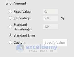
However, we can also add custom error bar if we want. In the above picture, we can see all the Error Bar Types in Excel.
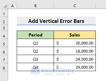
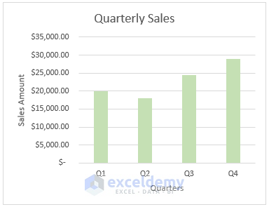
To illustrate, we’ll use a sample dataset as an example. For instance, the following dataset represents 4 periods and the Sales of a company. Accordingly, we’ll insert a 2-D chart containing these data values and add Vertical Error Bars in Excel. Therefore, follow the steps below to perform the task.
STEP 1: Inserting Column Chart in Excel
- Firstly, select the range B5:C8.
- Then, go to the Charts section in the Insert tab.
- After that, select the 2-D Column Chart or any other chart type.
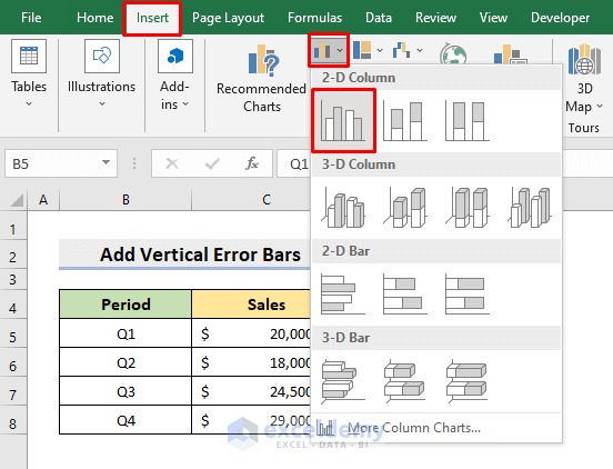
- As a result, you’ll get a column chart like it’s displayed below.
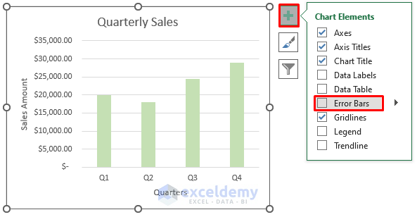
STEP 2: Adding Vertical Error Bars in Excel Column Chart
- Now, click the chart. Thus, you’ll see a Plus (+) icon on the right-hand side as demonstrated below.
- Next, press the icon.
- Consequently, it’ll return the Chart Elements box.
- There, check the box for Error Bars.
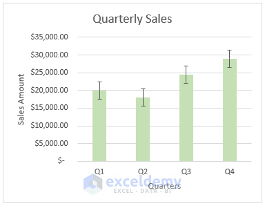
- Hence, you’ll notice the desired vertical error bars in the column chart.
How to Format Vertical Error Bars in Excel
Additionally, we can format the error bars as per our requirements. So, learn the following steps to carry out the operation.
STEPS:
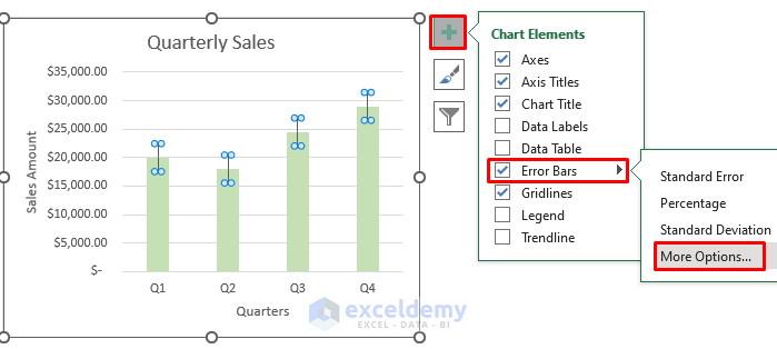
- Select the chart first.
- Afterward, click the Plus (+) icon and choose More Options from the Error Bars.
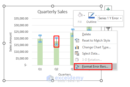
- To get the Format Error Bars pane in another process, select the error bars (inside the chart) and right-click on the mouse.
- Choose Format Error Bars from the list.
- As a result, it’ll return the Format Error Bars pane on the right side of the Excelworksheet.
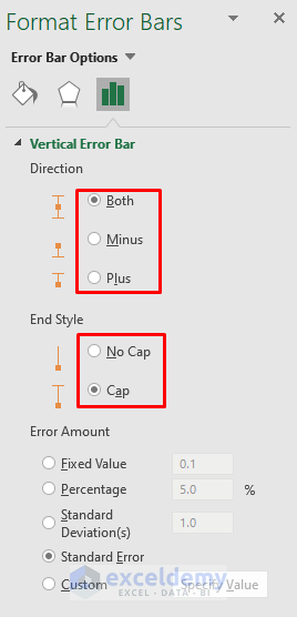
- Here, you can modify the Direction, End Style, etc.
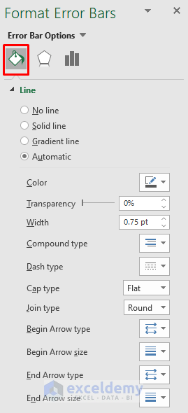
- Moreover, you can modify the Line.
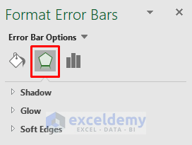
- In a similar way, modify the Shadow, Glow, and Soft Edges.
How to Add Vertical Error Bars in Excel 2010 or Earlier Versions
For adding Vertical Error Bars in earlier versions of Excel, follow the process below.
STEPS:
- First of all, select the chart. This will activate the Chart Tools tab.
- Afterward, go to Layout ➤ Error Bars.
- Lastly, select your desired error bar from the drop-down.
How to Delete Error Bars in Excel
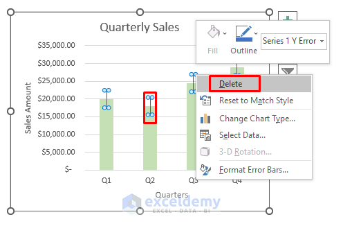
Finally, we may also want to erase the error bars. Learn the process to Delete the Vertical Error Bars in Excel.
STEPS:
- In the beginning, select the chart.
- Then, right-click on the mouse.
- At last, choose Delete.
Read More: How to Add Error Bars in Excel
Download Practice Workbook
Download the following workbook to practice by yourself.
Conclusion
Henceforth, you will be able to Add Vertical Error Bars in Excel following the above-described procedures. Keep using them and let us know if you have more ways to do the task. Don’t forget to drop comments, suggestions, or queries if you have any in the comment section below.
Related Articles
- How to Add Individual Error Bars in Excel
- How to Add Standard Deviation Error Bars in Excel
- How to Add Horizontal Error Bars in Excel
- How to Remove Horizontal Error Bars in Excel
- How to Graph Uncertainty in Excel
<< Go Back To Error Bars in Excel | Excel Chart Elements | Excel Charts | Learn Excel
Get FREE Advanced Excel Exercises with Solutions!
