How to Add Custom Error Bars in Excel (2 Examples)

Excel Error Bars on charts give a more complete perspective of the given data and enable citizens to see the edges or faults in the data. They show the accuracy of a measurement. There may be circumstances when a data point has a level of fluctuation when shown in a chart. If you need to display this type of data, where there is always some unpredictability and the final number might be somewhat higher or lower, we might use Error Bars in Excel Charts. In this article, we will show you how to add custom error bars in Excel.

What Are Error Bars in Excel?

Error Bars are visual portrayals of variations in the dependent variable that are used to highlight the error or disagreement in a given data point on the chart. They provide a basic indication of exact measurements or the distance the real (error-free) value may be from the value obtained.

Error bars can be added to 2-D bar, column, line, and area graphs, XY (scatter) plots, and bubble charts in Microsoft Excel. Transverse and longitudinal error bars can be presented in graphical representations and bubble charts. Error bars can be shown as a fixed value, standard error, standard deviation, and percentage.

Add Custom Error Bars in Excel: 2 Examples

Custom error bars are a subcategory of error bars. In this article, we will learn how to construct a customized error bar and add error bars specifically for a certain observed value. We may specify our list of data comprising formulae to generate the error bars on the chart by utilizing Custom Error Bars in Excel. The positive and negative error ranges can be defined. We may use many functions to obtain the mean of data, such as the AVERAGE function, and the STDEV.P function to obtain the standard deviation. There are two possibilities for using custom error bars:

Data points have similar variance.
Data points have dissimilar variances.

We will demonstrate both scenarios in this article. So, let us get started.

1. Excel Custom Error Bars with Similar Error Values for All Data Points

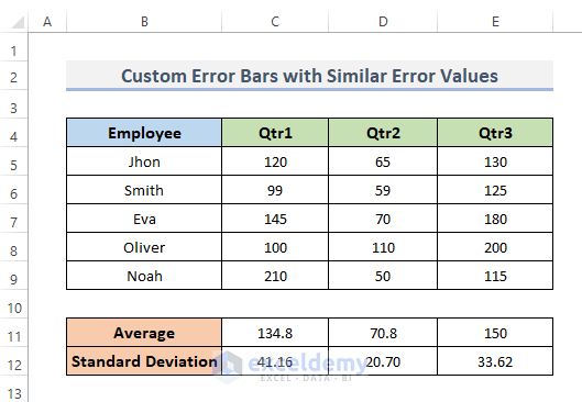
To add custom bars with the same variance for all data points, we are going to use the following dataset. The dataset contains a company’s quarterly sales. This includes some employee names and the sales of quarters 1, 2, and 3. We generated the averages (C5:C9), (D5:D9), and (E5:E9) of each quarter using the AVERAGE function for placing those on the bar chart. We also used the STDEV.P function to calculate the standard deviation for each column (C5:C9), (D5:D9), and (E5:E9). And now you want to show those statistics as standard deviation error bars in the bar chart.

For this, we need to follow the procedures shown below.

STEPS:

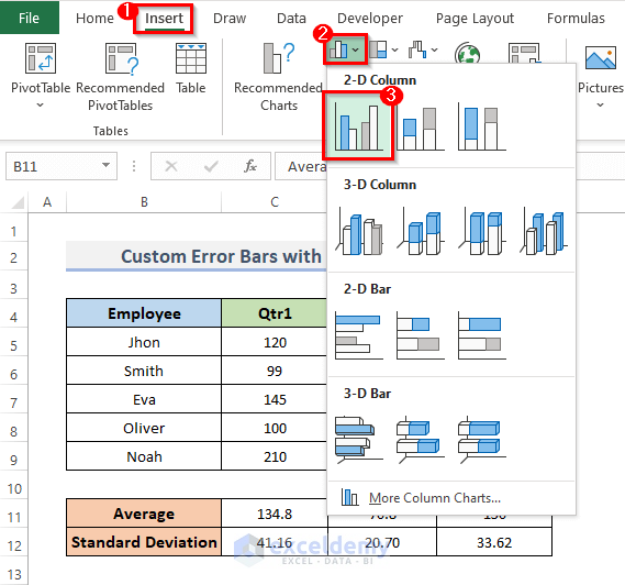
Firstly, select the averages to plot those averages in the bar chart. So, we select cell B11:E11.
Secondly, go to the Insert tab from the ribbon.
Thirdly, in the Charts category, click on the Insert Column or Bar Chart drop-down menu and choose the first chart, Clustered Column from the 2-D Column.

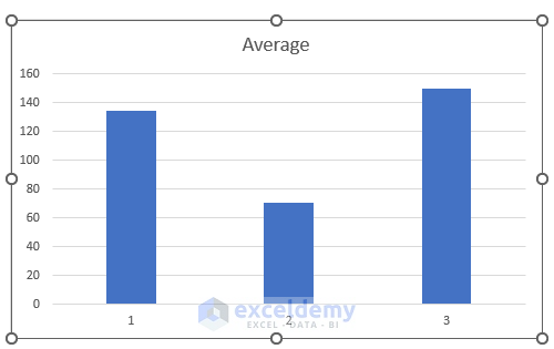
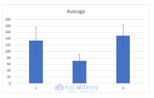
Then, you can see the data charts are inserted for better visualization. And the name of the chart is “Average”.

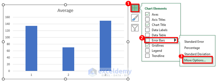
Now, to add custom error bars, click on the chart and go to the Chart Elements which is just beside the chart and the icon for the Chart Elements is a plus (+) sign.
Next, to the right of the Error Bars option, pick the black triangle indicator and then choose More Options.

This will open the Format Error Bars dialog on the right side of your spreadsheet.
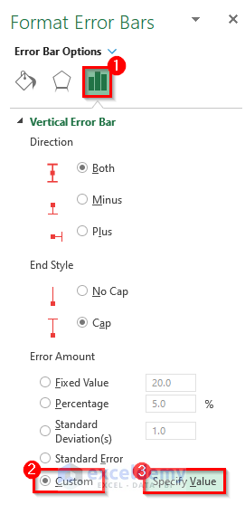
From the Error Bars Options, click on the chart symbol.
In the Error Amount option, choose Custom and click on the Specify Value beside the Custom option.

Therefore, this will display the Custom Error Bars dialog.
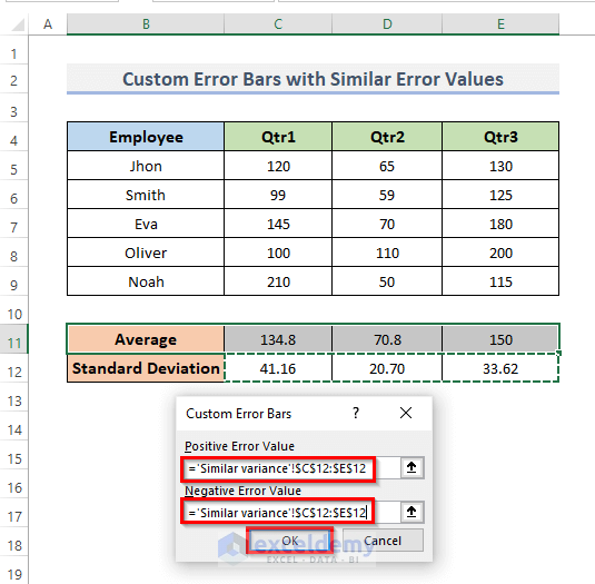
Here, for Positive Error Value, select the range that contains the standard deviation by clicking on the range selector icon.
As we add the custom error bars with similar error values, so, for Negative Error Value we again select the range that contains the standard deviation by clicking on the range selector icon.
Finally, click on the OK button to complete the procedure.

And that’s it! Based on the value of the standard deviation that we have chosen; the preceding steps will generate custom error bars for each data point.

Read More: How to Add Error Bars in Excel

2. Create Custom Error Bars If All Data Points Have Dissimilar Variance in Excel

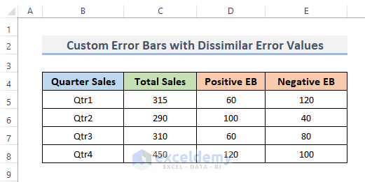
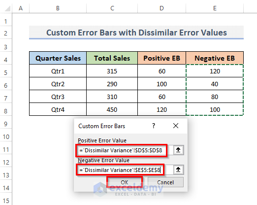
To add custom bars with different variability for all data points, assume that we are using the following dataset. The dataset has some quarter sales and total sales in each quarter, as well as the Positive Efficiency Bar (EB) and the Negative Efficiency Bar (EB) to plot the chart and add the custom error bars perfectly.

We must follow the measures outlined below to do this.

STEPS:

Similarly, as before, to begin with, pick the ranges to plot the bar chart. As a result, we chose cell B4:C8.
Then, from the ribbon, select the Insert tab.
Next, under the Charts group, select Clustered Column from the 2-D Column of the Insert Column or Bar Chart drop-down menu.

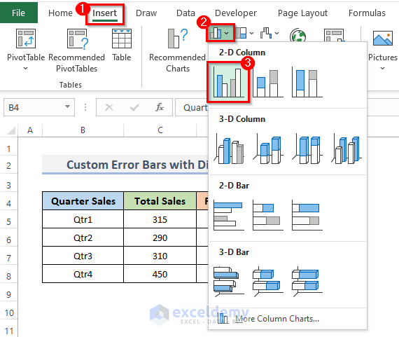
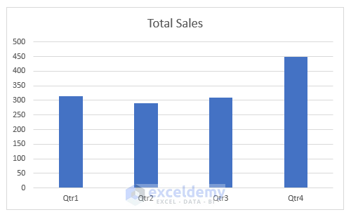
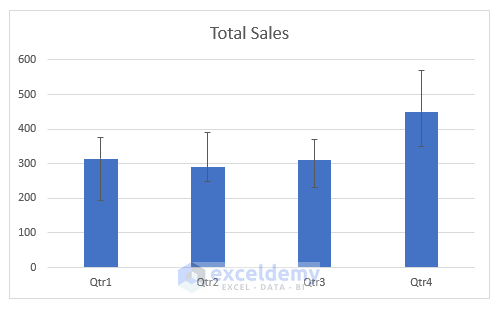
This will place the data charts for greater viewing. And the chart’s name is “Total Sales”.

To add custom error bars, click on the chart and then go to the Chart Elements, which is directly beneath the chart and has a plus (+) symbol as its icon.
Further, to the right of the Error Bars option, select the black triangle indication to select More Options.

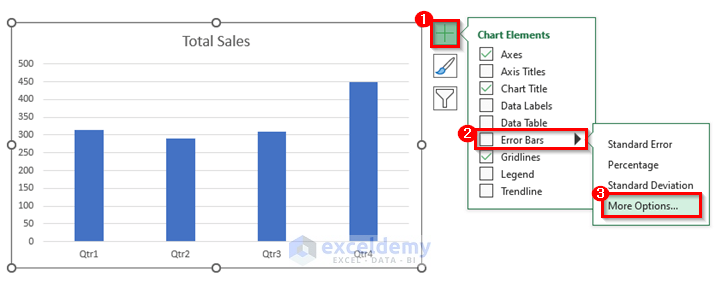
Thus, The Format Error Bars dialog will appear on the right side of your spreadsheet.
Now, select the chart symbol from the Error Bars Options menu.
Furthermore, under the Error Amount section, select Custom and click the Specify Value button next to the Custom option.

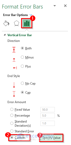
The Custom Error Bars dialog will appear.
For Positive Error Value, click on the range selector icon to select the range containing the positive eb (D5:D8).
As we add custom error bars with different error values, we choose the range that contains the negative eb (E5:E8) by clicking on the range selector icon for Negative Error Value.
Finally, click the OK button to finish the process.

And there you have it! The previous steps will build bespoke error bars for each data point based on the value of different variables that we have chosen.

Download Practice Workbook

You can download the workbook and practice with them.

Add Custom Error Bars.xlsx

Conclusion

The above methods will assist you in how to add custom error bars in Excel. Hope this will help you! If you have any questions, suggestions, or feedback, please let us know in the comment section.

<< Go Back To Error Bars in Excel | Excel Chart Elements | Excel Charts | Learn Excel

Get FREE Advanced Excel Exercises with Solutions!