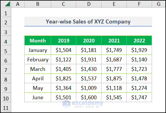
Method 1 – Input a Dataset with Necessary Components
- Insert a dataset that will be populated with the necessary components. We have taken a dataset of Year-wise Sales of XYZ Company.
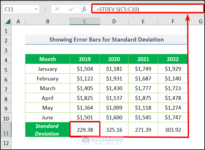
Method 2 – Calculate Standard Deviation
- Calculate the standard deviation of your dataset by the STDEV.S function.
- Go to cell C11 and write up the formula.
=STDEV.S(C5:C10)
The above syntax finds the standard deviation of cell range C5:C10.
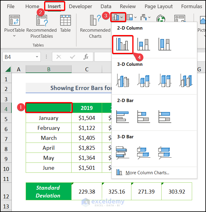
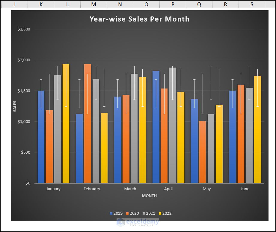
Method 3 – Insert Bar Chart
- Select cell B4 after removing the column header.
- Navigate to the Insert tab >> choose Insert Column or Bar Chart >>pick Clustered Column.
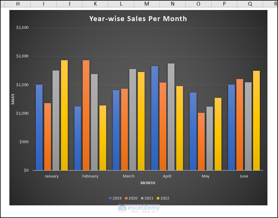
It will create a bar chart with multiple bars like the image below.
Method 4 – Plot Error Bars to Show Standard Deviation
- Select the plot area. Click on the ➕ (plus sign) which represents the Chart Elements. Check the Error Bar and choose Standard Deviation.
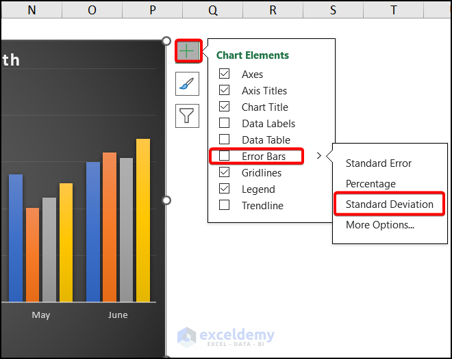
Get the chart with the standard deviation error bars.
Method 5 – Customize Error Bars
- Customize the error bars. Click on any error bar and apparently, Format Error Bars appear.
- Choose the Custom command in the Error Amount option and select the Specify Value.
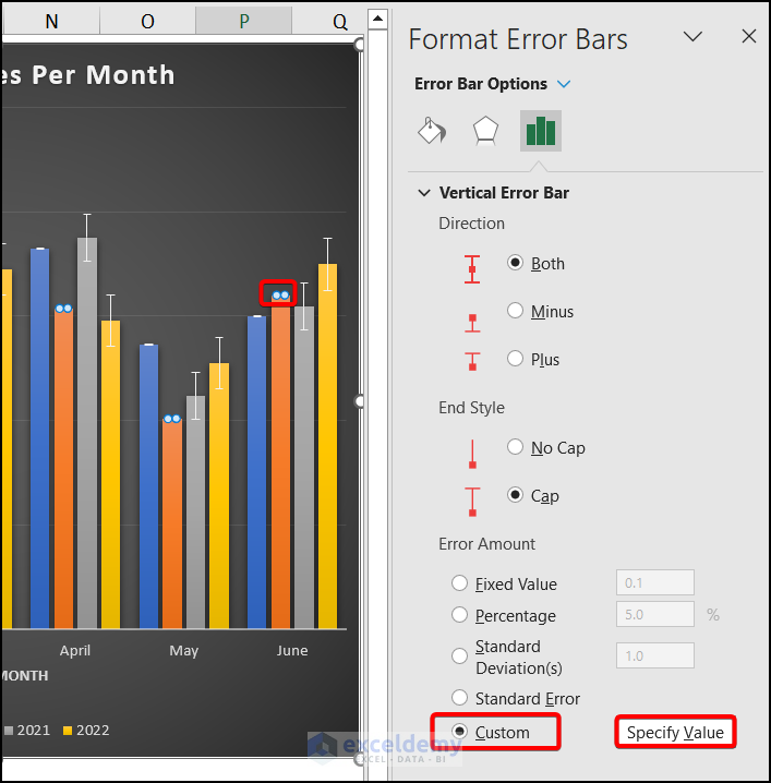
- The Custom Error Bars window appears. Put the Positive and Negative Error Value to 20.
- Hit OK.

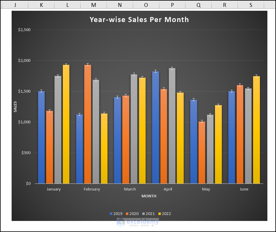
Get the standard deviation error bars like the image below.
Download Practice Workbook
Download the following practice workbook. It will help you to realize the topic more clearly.
Related Articles
- How to Add Error Bars in Excel
- How to Add Custom Error Bars in Excel
- How to Add Horizontal Error Bars in Excel
- How to Graph Uncertainty in Excel
<< Go Back To Excel Chart Elements | Excel Charts | Learn Excel
Get FREE Advanced Excel Exercises with Solutions!
