Horizontal error bars in charts that we create help us a lot to see margins of error and show standard deviations. But sometimes we need to get rid of it, and if you don’t know it, then you have come to the right place. Here, I’ll show the 4 quick methods to remove horizontal error bars in Excel with proper illustrations.
How to Remove Horizontal Error Bars in Excel: 4 Ways
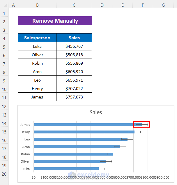
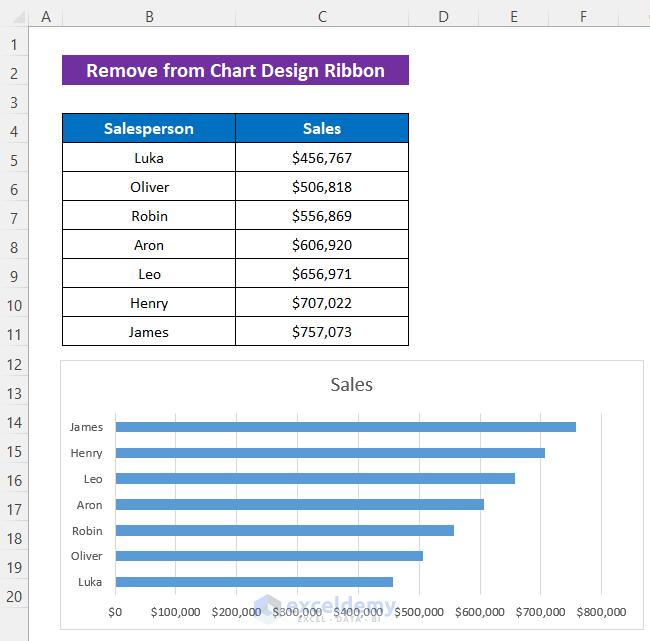
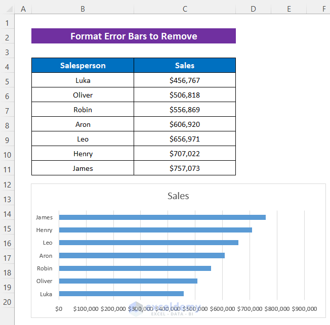
Let’s get introduced to our dataset first. It represents some salespersons’ sales. I have created a chart from the data and look, there are horizontal error bars in my chart.
READ MORE: How to Add Error Bars in Excel
1. Manually Remove Horizontal Error Bars in Excel
First, we’ll apply the manual method to remove horizontal error bars using the DELETE key from the keyboard.
Steps:
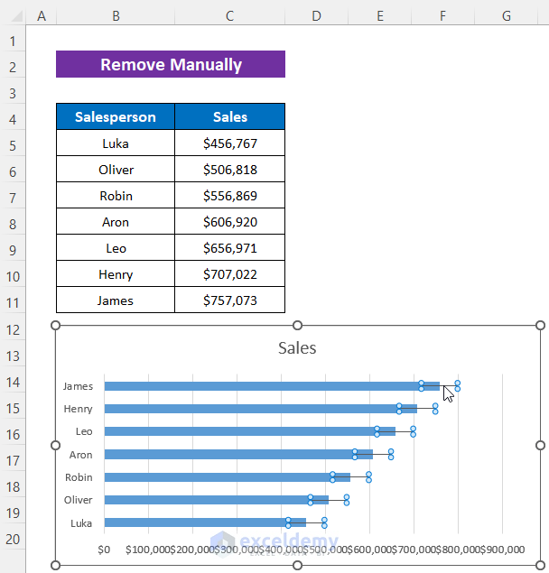
- Click on any horizontal error bar from your chart.
- Then, just press the DELETE key.
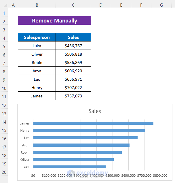
Now you see, all the horizontal error bars are gone from the Excel chart.
2. Remove Horizontal Error Bars from Chart Elements
There is an option in the Excel chart named ‘Chart Element’; from there we can easily delete the horizontal error bars. Let’s see how to do it.
Steps:
- Select the chart by clicking it and then you will get a plus icon on the top right side of your chart, which is the Chart Elements
- Just click on it and unmark Error Bars from the appeared list.
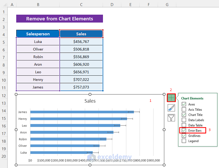
Soon after you will see that no horizontal error bars are remaining in your chart.

READ MORE: How to Add Custom Error Bars in Excel
3. Delete Horizontal Error Bars from Excel Chart Design Ribbon
You will get the same Chart Elements command in the Excel Chart Design ribbon, too. So of course, by using it, you will be able to remove the error bars.
Steps:
- First, select your chart, and then the Chart Design ribbon will be visible in the ribbon bar.
- Later, click as follows from the ribbon: Add Chart Element > Error Bars > None.
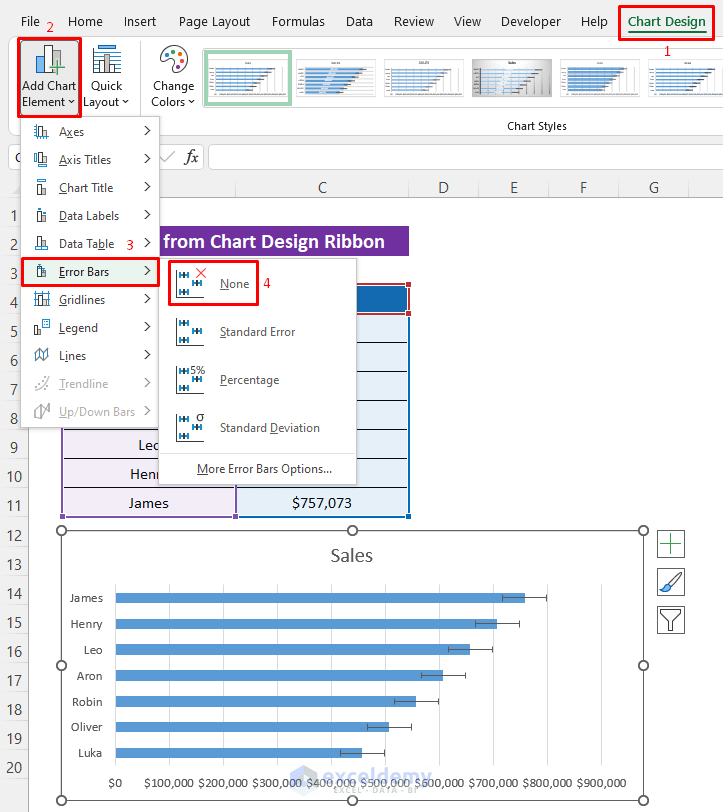
Now, see the image below; no horizontal error bars.
READ MORE: How to Add Individual Error Bars in Excel
4. Format Error Bars in Excel to Erase Horizontal Error Bars
The above methods were the direct ways to remove error bars. Here, we’ll learn two indirect ways that will not permanently remove the horizontal error bars but will seem like they have been removed.
4.1. Mark No Line to Delete Horizontal Error Bars
By formatting the error bars, we can change the line format of the bar, and we’ll choose No Line for our task.
Steps:
- Right-click on any of the error bars.
- Next, select Format Error Bars from the Context menu.
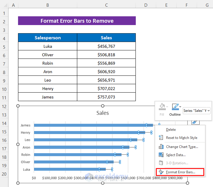
Soon after the Format Error Bars dialog box will appear on the right side of your Excel window.
- Click on Fill & Line icon.
- Later, mark No Line.
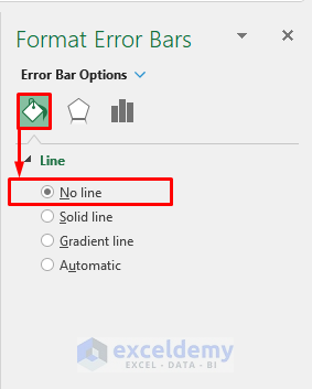
Now see, the lines from the error bars are removed.

If you click anywhere outside of your Excel chart then it will look like there are no horizontal error bars.
4.2. Use 100% Transparency to Hide Horizontal Error Bars
We can change the line transparency of the bars by formatting. So, if we set the transparency to 100%, then the bar will seem like it vanished.
Steps:
- First, open the Format Error Bars following the previous section then click on Fill & Line.
- Then, from the Transparency bar, just set it to 100%.
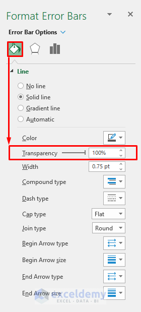
The bars are now fully transparent, so you won’t see them anymore.
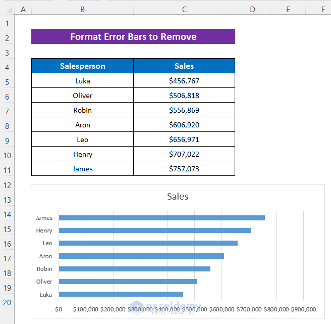
Though it’s not the conventional way of removing the error bars, it’s only hiding the bars, still, it may help you in your time of need.
Download Practice Workbook
You can download the free Excel workbook from here and practice on your own.
Conclusion
I hope the procedures described above will be good enough to remove horizontal error bars in Excel. Feel free to ask any question in the comment section and please give me feedback.
Related Articles
- How to Add Vertical Error Bars in Excel
- How to Add Horizontal Error Bars in Excel
- How to Add Standard Deviation Error Bars in Excel
- How to Graph Uncertainty in Excel
<< Go Back To Error Bars in Excel | Excel Chart Elements | Excel Charts | Learn Excel
Get FREE Advanced Excel Exercises with Solutions!
