Excel Worksheets Basics – A Beginner’s Guide

Excel worksheets are like digital pages where you can type, calculate, and analyze data. They are divided into rows and columns to help you keep things organized.

⏷What Is an Excel Worksheet
⏷Create an Excel Worksheet
⏷Add New Worksheet
⏷Rename a Worksheet
⏷Activate a Worksheet
⏷Move a Worksheet Tab
⏷Change Excel Sheet Directions
⏷Delete a Worksheet
⏷Copy a Worksheet
⏷Hide and Unhide Sheet
⏷Group and Ungroup Worksheets
⏷Protect Cells in an Excel Worksheet
⏷Change Sheet Tab Color
⏷Compare Excel Sheets
⏷Zoom In and Out
⏷Resize Excel Window
⏷Limit Excel Sheet Size
⏷Split Excel Sheet
⏷Count Total Sheets in an Excel Workbook

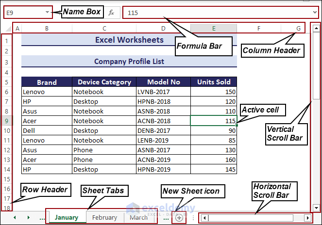
What Is an Excel Worksheet?

An Excel worksheet is a grid-based document used for organizing and analyzing numerical data.

The worksheet consists of rows and columns, forming cells where users can input and manipulate data.

Each intersection of a row and a column is called a cell, and each cell can contain text, numbers, formulas, or functions.

Users can perform various calculations, create lists or charts, and organize data in a structured manner.

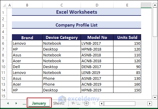
How to Create an Excel Worksheet?

To create an Excel worksheet, follow the steps below.

• Open Microsoft Excel and select Blank workbook.

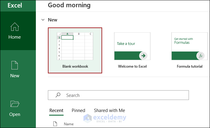
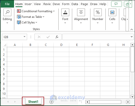
• The blank Excel worksheet is showcased as Sheet1.

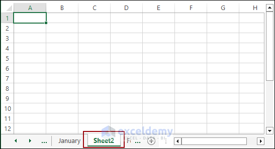
How to Add New Worksheets in Your Workbook?

To insert a new worksheet in an Excel workbook:

• Press the plus (+) symbol at the bottom.

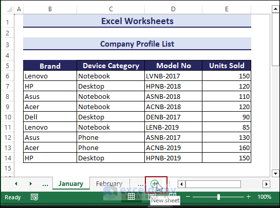
• A new sheet will open.

Note: You can insert a new worksheet by Pressing Shift + F11.

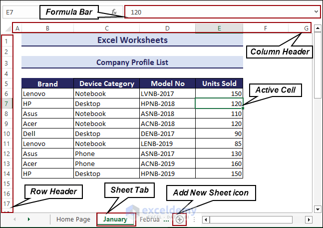
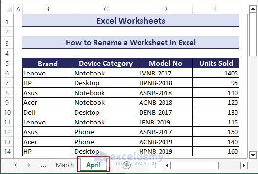
How to Rename a Worksheet?

You can rename a worksheet in Excel by using the Context Menu.

• Right-click the sheet name >> A Context Menu will appear >> Select Rename.

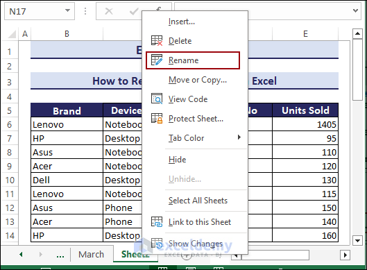
• Sheet2 is renamed to April.

You can also rename multiple sheets.

How to Activate a Worksheet?

To make a worksheet active,  left-click the Sheet Name.

Left Clicking the Sheet Name

• Click any sheet tab to make it active.

Using the Keyboard and the Mouse

Ctrl + Left Click: You can Scroll to the last sheet

Right Click: You can See all sheets

To activate  January, right-click the right arrow.

• In  the Activate window >> Select January >> OK.

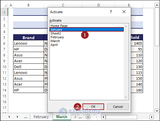
• You can activate January using the keyboard shortcut.

How to Move a Worksheet Tab in an Excel Workbook?

To move  January:

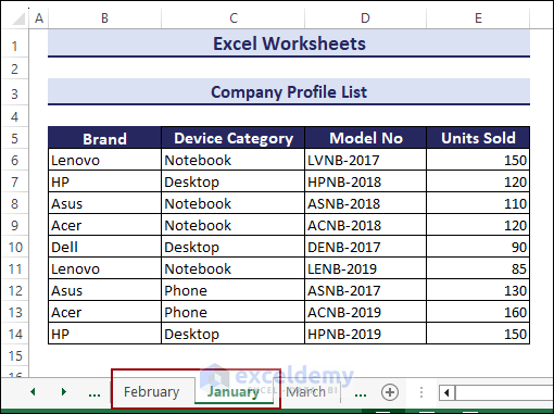
• Left-click January and hold. Release it after February.

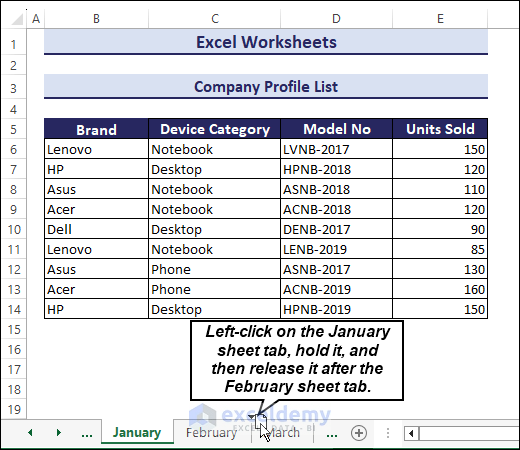
• January will be displayed after February.

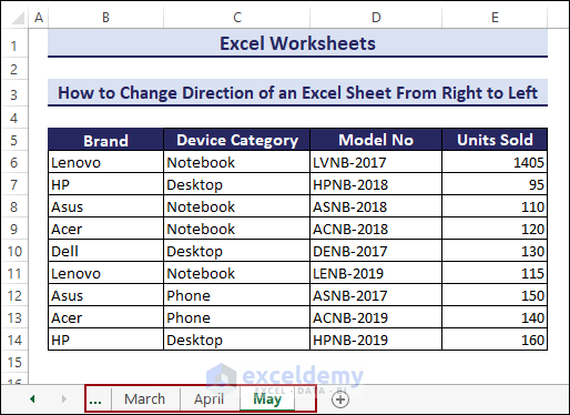
How to Change the Direction of an Excel Sheet From the Right to the Left or from the Left to the Right?

The Excel sheet direction is from the left to the right by default.

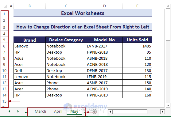
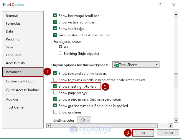
1. Changing the Excel Sheet Direction from Left-to-Right to Right-to-Left

• Go to the File tab >> Options.
• In the Excel Options dialog box >> Select Advanced.
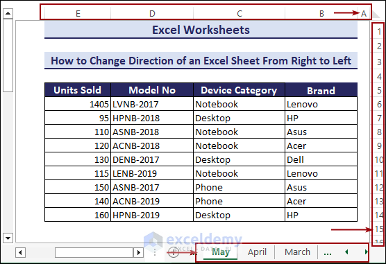
• In Display options for this worksheet  >> Check  Show sheet right-to-left  >> OK.

• You can also change the directions of the Excel sheet from the left to the right.

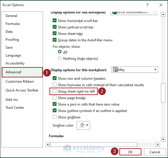
2. Changing the Excel Sheet Directions from Right-to-Left to Left-to-Right

• Press Alt + F + T  to open Excel Options >> Select  Advanced.
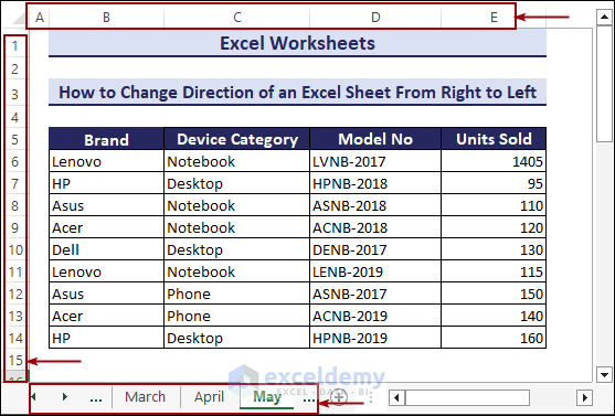
• Go to Display options for this worksheet>> Uncheck Show sheet right-to-left >> OK.

• The direction was changed from the right to the  left.

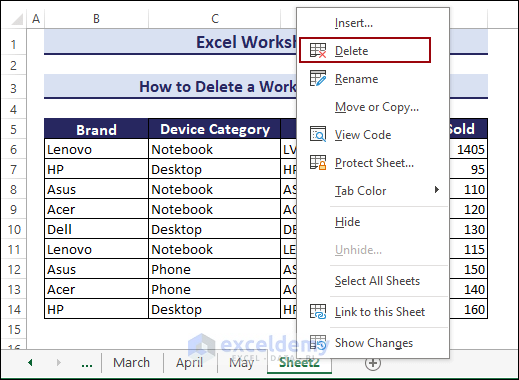
How to Delete a Worksheet in Excel?

To delete a worksheet, for example, Sheet2:

• Right-click the sheet tab >> Click  Delete.

• In the Microsoft Excel warning window >> Delete.

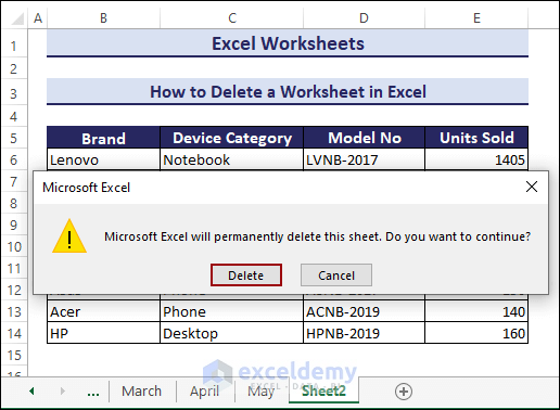
• Sheet2 was deleted.

You can also delete the multiple worksheets.

How to Copy a Worksheet in Excel?

To copy a sheet, right-click.

Within the Same Workbook

• Select January  >> Right-click the sheet tab >> Select Move or Copy .

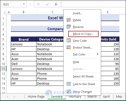
• In the Move or Copy dialog box >> Select March.
• Check Create a copy >> Click OK.

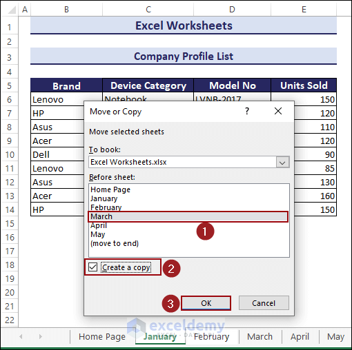
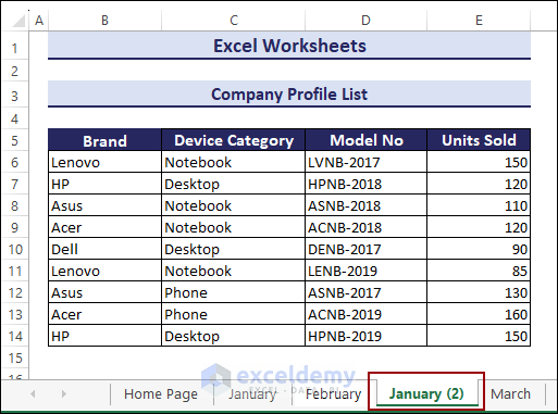
• The copied sheet (January (2)) is before March.

To Another Workbook

Open both workbooks. You will copy  January (2) in the Excel Worksheets.xlsx workbook to Scrolling in Excel.xlsm workbook.

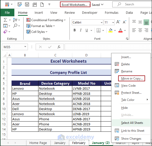
• In the Move or Copy dialog box >> Select Scrolling in Excel.xlsm in To book.
• In Before sheet, select Smooth Scrolling.
• Check  Create a copy >> Click OK

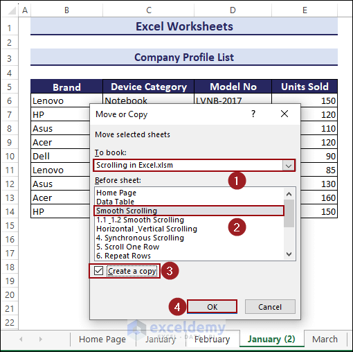
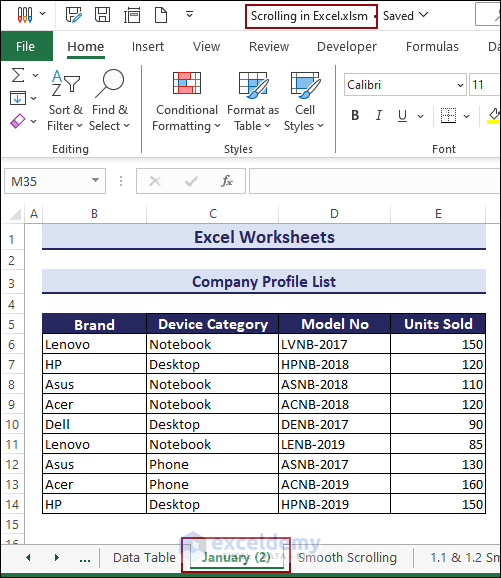
• January (2) in the Excel Worksheets.xlsx workbook was copied to Scrolling in Excel.xlsm workbook before the Smooth Scrolling sheet.

How to Hide and Unhide Sheets in Excel?

The simplest way to hide and unhide worksheets from workbook is to right-click the worksheet.

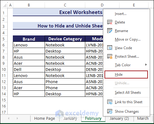
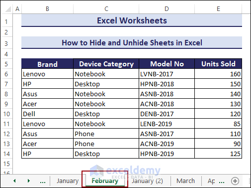
Hiding a Sheet in Excel

• Select February and right-click the sheet name >> In the Context Menu  >> Select Hide.

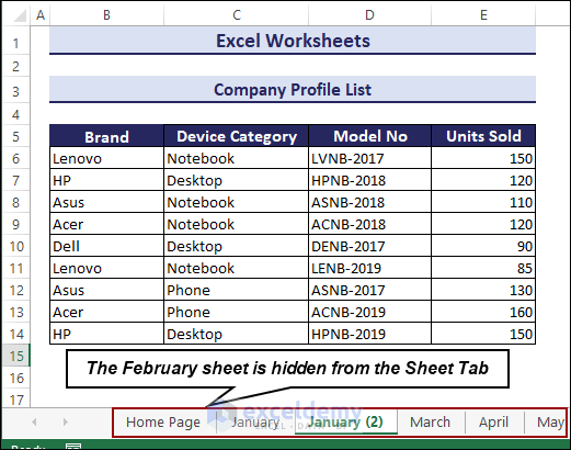
• February is hidden from the sheet tab.

Unhiding Sheet in Excel

• Select any sheet >> Right-click the sheet name >> In the Context Menu >> Choose Unhide.

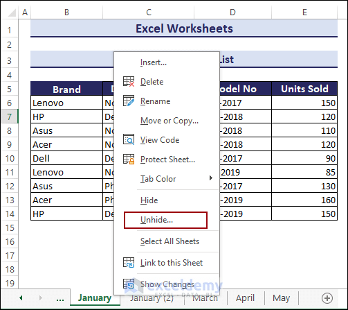
• In the Unhide dialog box >> Select February from the Unhide one or more sheets drop-down menu >> OK.

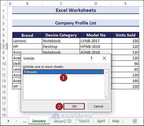
• Unhide the hidden sheet(s).

How to Group and Ungroup Worksheets in Excel?

You can group and ungroup the adjacent and nonadjacent worksheet tabs. If you change any data on any grouped sheet tab, it will automatically change the data on every sheet tab.

Grouping Adjacent and Nonadjacent Worksheets

Non-adjacent worksheet tabs: Click any sheet tab >> Press and hold Ctrl>> Select the sheets you want to group.

Adjacent worksheet tabs: Select any sheet tab >> Press and hold Shift, click the leftmost or rightmost sheet tab.

Ungrouping Adjacent and Nonadjacent Worksheets

Right-click any grouped sheet tabs >> Choose  Ungroup Sheets in the Context Menu.

Note: You can also ungroup the worksheets by clicking any unselected sheet tab.

How to Protect Excel Worksheet?

Follow these steps:

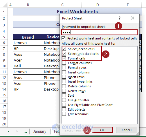
• Right-click the sheet tab >> Choose Protect Sheet in the Context Menu.

• In the Protect Sheet window  >> Enter a password in Password to unprotect sheet.
• Choose your options in Allow all users of this worksheet to >> OK.

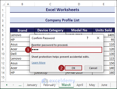
• In the Confirmed Password dialog box >> Reenter the password in Reenter password to protect >> OK.
• March is protected with a password.

• TO check whether the sheet is protected, select C11 and Enter random data. A warning message will be displayed, confirming the sheet is protected.

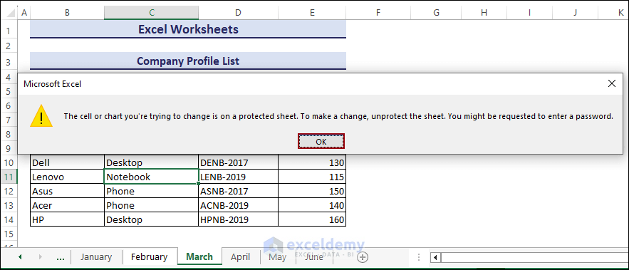
Click here to enlarge image

How to Change a Worksheet Tab Color in Excel?

You can change the sheet tab color in Excel. By default, the color of a sheet tab is white. You can change it to any color you want. Observe the GIF below.

How to Compare Excel Sheets?

1. Compare Excel Sheets with the View Tab

You can use the View Side by Side feature from the View tab to compare Excel sheets in the same workbook and in different workbooks.

In the Same Workbook

• Go to the View tab >> Window  >> Click  New Window.

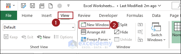
• A new workbook window will open.
• By default, Excel displays two separate Excel windows horizontally.
• To display the windows vertically. Go to the View tab >> Window >> Click Arrange All.
• In the Arrange Windows dialog box  >> Check Vertical >> OK.

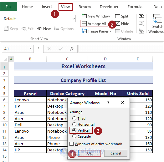
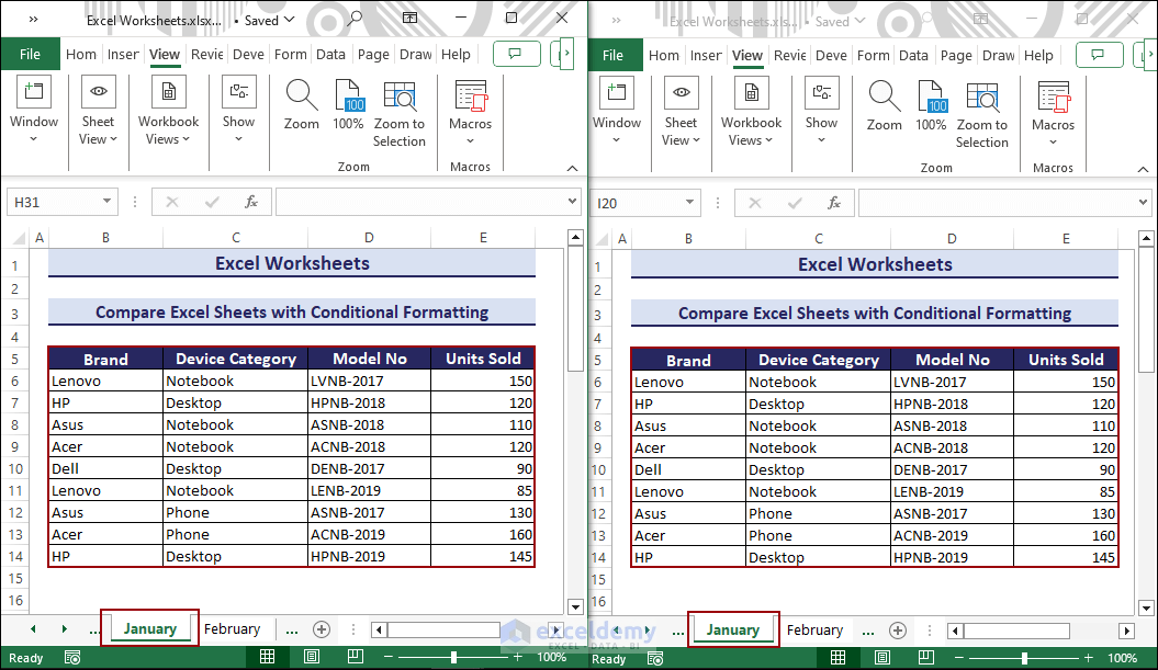
• Both workbook windows are vertically displayed.

Click here to enlarge image

• To scroll both windows at a time, enable Synchronous Scrolling.
• Follow the steps in the GIF.

Click here to enlarge image

Different Workbooks

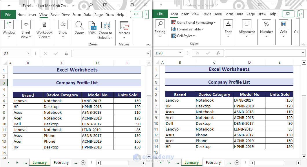
You can compare different workbooks at a time using the View Side by Side feature and the Synchronous Scrolling command of Excel. The workbooks must be open.

• Go to View tab >> Window >> Select View Side by Side.

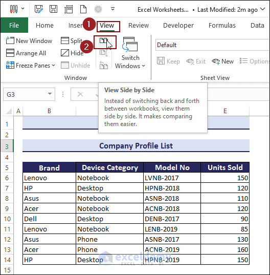
The Synchronous Scrolling command will be enabled automatically for both workbooks.

Click here to enlarge image

• Select any cell and scroll to compare both workbooks.

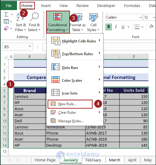
2. Compare Excel Sheets with Conditional Formatting

You can compare Excel sheets and highlight the different values with conditional formatting.  January and February will be compared here.

Follow these steps:

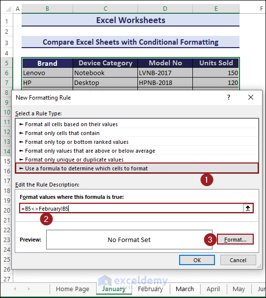
• Select B5:E14 >> Go to the Home tab >> Styles >> Conditional Formatting >> Select New Rule.

• In the New Formatting Rule dialog box >> In Format values where this formula is true, select Use a formula to determine which cells to format.
• Enter the following formula:

• Click Format…

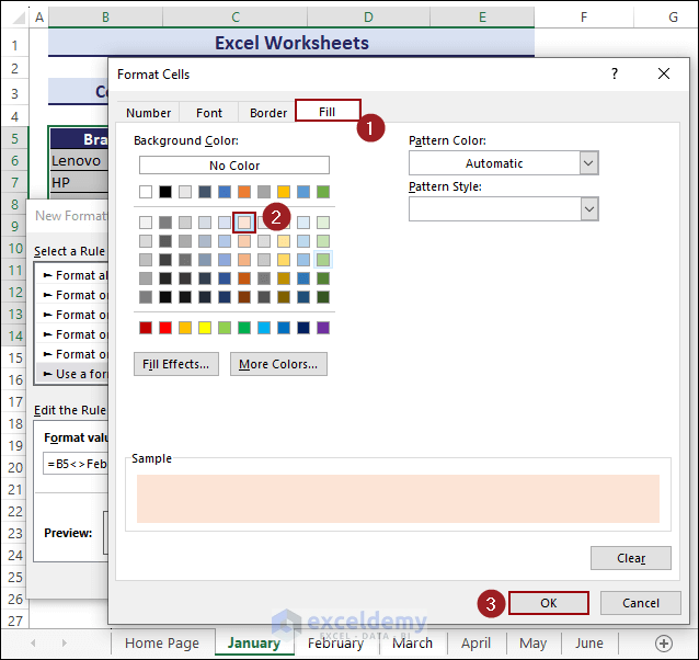
• In Format Cells, go to Fill and choose a color.
• Click OK.

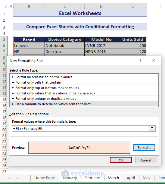
• In New Formatting Rule, click OK.

• Different values between January and February are highlighted.

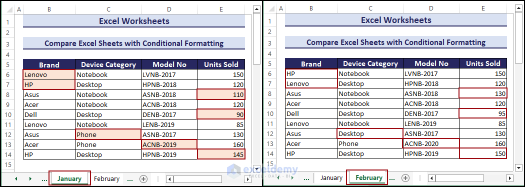
Click here to enlarge image

How to Zoom In and Out in Excel Worksheets?

You can Zoom In or Zoom Out. Observe the GIF.

How to Resize the Excel Window or View Excel in Full Screen?

You can use the Maximize and Minimize options.

To enable Full Screen View press Ctrl + Shift + F1 keys.

Click here to enlarge image

To resize the Excel sheet window, Drag the sheet window. Observe the GIF.

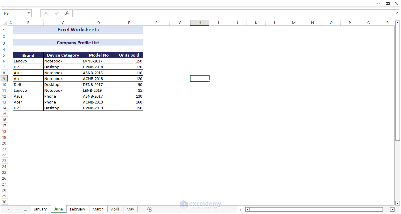
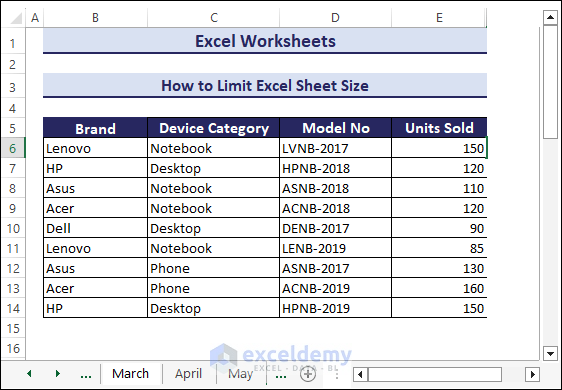
How to Limit Excel Sheet Size?

Limiting Excel sheet size means preventing others from viewing additional rows and columns.

1. Hide Unused Rows and Columns

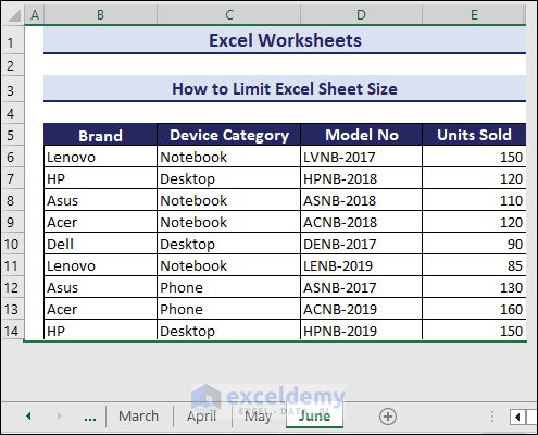
Here, rows up to 14 and columns up to  E in the June sheet will be hidden.

• Select any cell in column F. Here, F6 >> Press Ctrl + Shift + Right Arrow (→) to select the rest of the columns.
• Press Ctrl + 0 to hide columns.

• Columns are hidden.

• Select the entire row 15 >> Press Ctrl + Shift + Right Arrow (↓) to select the rest of the columns.
• Press Ctrl + 9 to hide the selected rows.

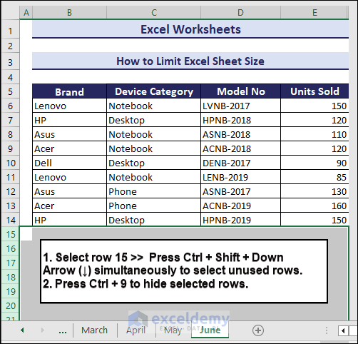
• Unused rows in June are hidden.

2. Using the Developer Properties Command to Limit Excel Sheet Size

• Go to the Developer tab >> Controls >> Properties command.
• In the Properties window >> Set scroll area in the ScrollArea. Here, $A$1:$E$20.
• Close the window (X).

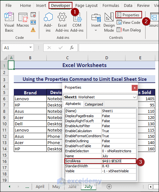
• Your Excel sheet is limited to the range $A$1:$E$20.

3. Using a VBA Code to Limit Sheet Size

Follow these steps:

• Press Alt + F11 to open the Microsoft Visual Basic for Applications window.
• Select Insert  >> Module.

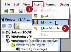
• In the VBA Module, enter the following code and run the macro.

Sub Limit_Sheet_Size()
Dim lss As Worksheet
Set lss = ActiveSheet
lss.ScrollArea = "$A$1: $E$20"
End Sub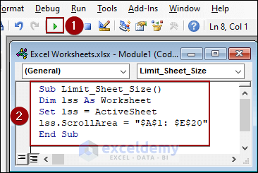

How to Split Excel Sheets?

To split screen or an Excel sheet within the same sheet, follow these steps:

• Select C9 >> Go to View >> Window >> Select Split.

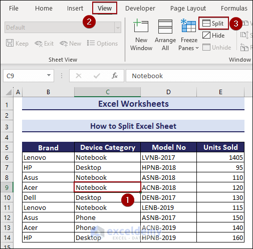
• Your sheet is split into four panes.

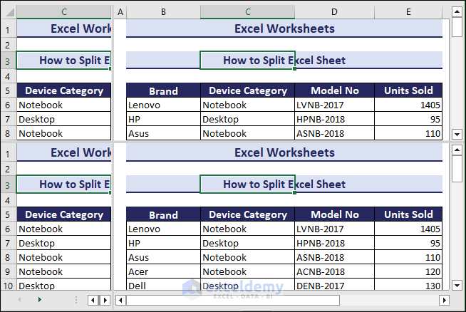
Observe the GIF.

How to Count the Number of Sheets in an Excel Workbook?

Use the SHEETS function to count the total number of sheets.

• In C5, enter the following formula and press Enter.

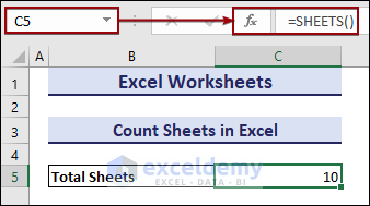
Download Practice Workbook

Excel Worksheets: Knowledge Hub

<< Go Back to Learn Excel