Looking for ways to show the percentage in 100 stacked column chart in Excel? Then this is the right article for you. You can show the percentage easily in a Pie Chart. However, it is not so straightforward for a Column Chart. Do not worry, we got you. In this article, we are going to show you 2 easy methods to show the percentage in the 100 stacked column chart in Excel.
Show Percentage in 100 Stacked Column Chart in Excel: 2 Suitable Examples
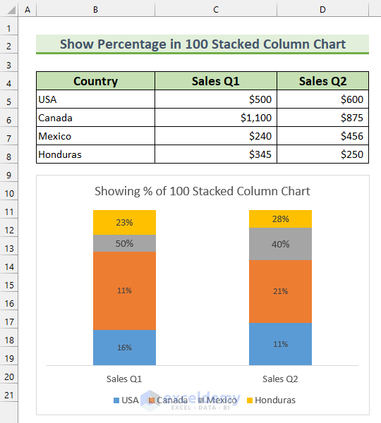
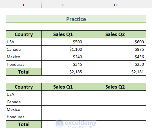
To demonstrate our methods, we have selected a dataset with 3 columns: “Country”, “Sales Q1”, and “Sales Q2”. Basically, we are showing the sales data by country for the first two quarters of the year 2022. We will use this data to construct a 100 stacked column chart and show the percentage in Excel. Here is a snapshot of the ultimate outcome of this article.
1. Using Value From Cells Feature to Show Percentage in 100 Stacked Column Chart
In this section, we will first find the total amount of sales using the SUM function. Then, we insert a basic 100 stacked column chart, which shows only values. After that, we will calculate the percentage of the sales. Lastly, using the Value From Cells feature, we will achieve the goal of showing the percentage in the 100 stacked column chart.
Steps:
- At first, select the cell range C9:D9 and type the following formula.
=SUM(C5:C8)
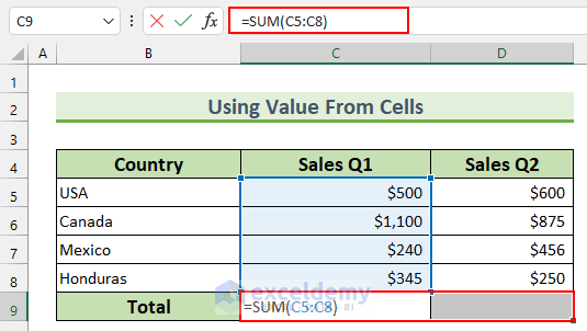
- Then, press CTRL+ENTER.
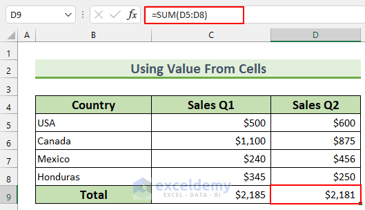
- This will autofill the formula and show us the total amount.
- Alternatively, you can select the cell range and press ALT+= to get the total.
- Next, select the cell range B4:D8.
- Afterward, from the Insert tab → Insert Column or Bar Chart → select 100% Stacked Column.
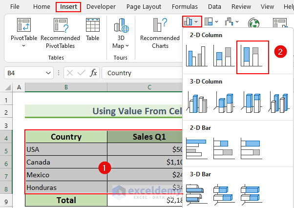
- So, we will get this basic chart.
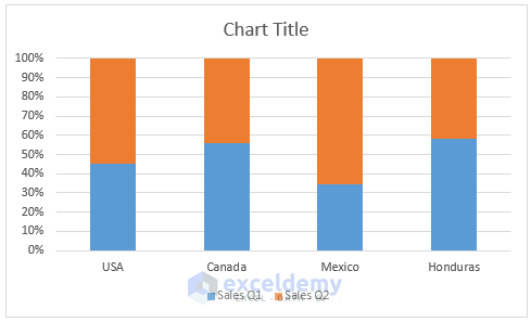
- Now, we will swap the row with the column.
- To do so, select the chart, and from the Chart Design tab, select Switch Row/Column.
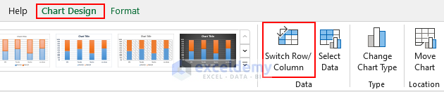
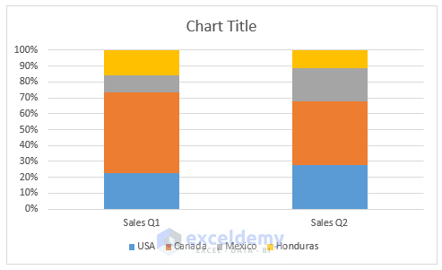
- Thus, our chart will change like this.
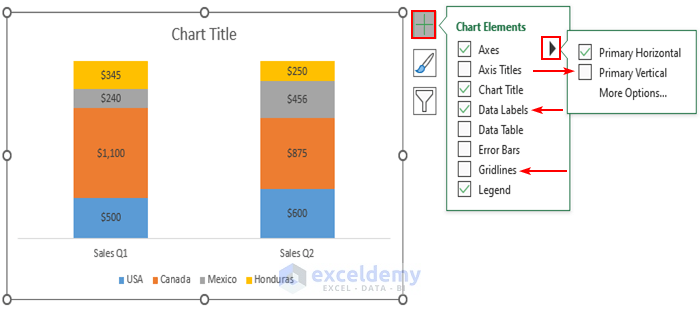
- Then, select the chart again and select Chart Elements.
- From the Axes, deselect Primary Vertical. This will hide the vertical axis.
- After that, select Data Labels.
- Then, deselect Gridlines. So, the gridlines will disappear.
- Now, we can see there are data labels but it does not show any percentage values. We are going to fix this next.
- Then, we copy and paste the original dataset to the cell range B11:D16 and delete all the numerical values.
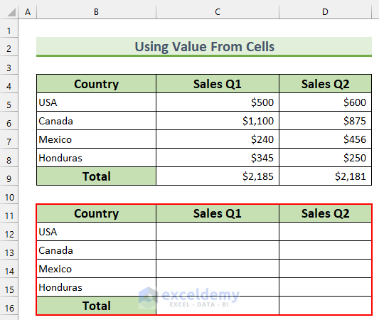
- After that, type the following formula in cell C12.
=C5/C$9
- Then, press ENTER and use the Fill Handle to autofill the formula to the rest of the cells. Remember to change these cell formats to percentages.
- Now, we move back to the chart and double-click on the first Data Label.
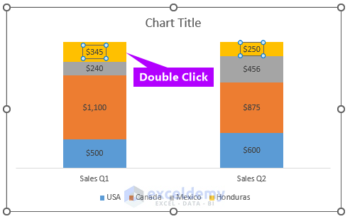
- Consequently, this will bring up the Format Data Labels box.
- Then, deselect Value and select Value From Cells.
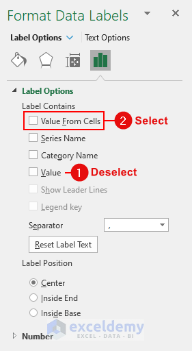
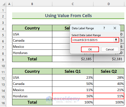
- So, another dialog box will pop up.
- The first Data Label is for Honduras, hence, we select the cell range C15:D15.
- After that, press OK.
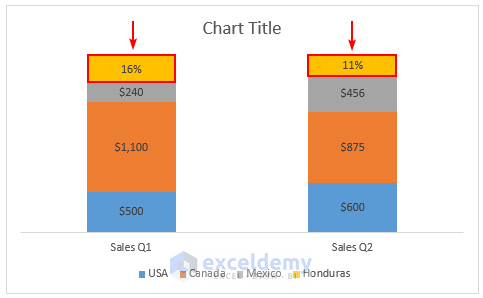
- By doing so, we will see the first Data Label showing percentages.
- Similarly, we will do for the rest of the Data Labels.
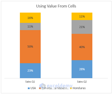
- Then, we added a title to the chart and increased the font size.
- Finally, our final step should look like this image.
2. Applying VBA to Show Percentage in 100 Stacked Column Chart
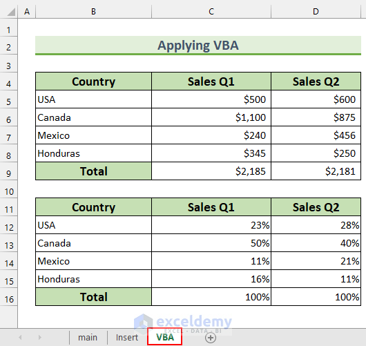
For the last method, we are going to apply an Excel VBA macro to show the percentage in 100 stacked column chart. Moreover, we can see that our dataset is in the “VBA” worksheet and we are using the same percentage dataset that we calculated in method 1.
Steps:
- To begin with, press ALT+F11 to bring up the VBA window.
- Alternatively, we can do it by selecting Visual Basic from the Developer tab.

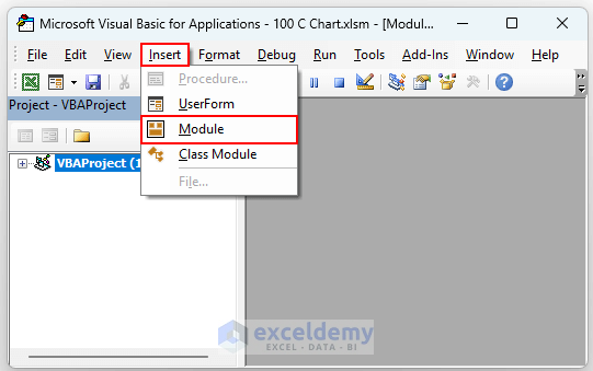
- Then, from Insert → select Module. We’ll type our code here.
- Then, type the following code.
Sub Show_Percentage_100_Stacked_Column_Chart()
    ActiveSheet.Shapes.AddChart.Select
    With ActiveChart
        .SetSourceData Source:=Range("VBA!$B$11:$D$15")
        .ChartType = xlColumnStacked100
        .PlotBy = xlRows
        .SetElement (msoElementPrimaryValueGridLinesNone)
        .SetElement (msoElementDataLabelCenter)
        .SetElement (msoElementPrimaryValueAxisNone)
        .HasTitle = True
        .ChartTitle.Text = "Applying VBA"
    End With
End Sub
VBA Code Breakdown
- First, we are calling our Sub procedure Show_Percentage_100_Stacked_Column_Chart.
- Next, we insert a chart in the Active Sheet.
- Then, we use the VBA With statement to set the properties of the Chart.
- Here, our data range is B11:D15, you need to change it according to your needs.
- Afterward, we make the gridlines from the graph disappear, swap rows with columns in the chart, and hide the vertical axis.
- After that, we add a Title to the Chart.
- Thus, this code works to create a 100 Stacked Column Chart.
- Afterward, save the module.
- Then, put the cursor inside the first Sub procedure and press Run.

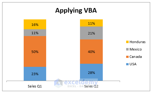
- So, our code will execute and it will create a 100 stacked column chart that shows the percentage.
Practice Section
We have added a practice dataset for each method in the Excel file. Therefore, you can follow along with our methods easily.
Download Practice Workbook
Conclusion
We have shown you 2 handy approaches to how to show the percentage in 100 stacked column chart in Excel. If you face any problems regarding these methods or have any feedback for me, feel free to comment below.
Related Articles
- How to Insert a Clustered Column Chart in Excel
- How to Create a 2D Clustered Column Chart in Excel
- How to Create a Stacked Column Chart in Excel
- How to Make a 100% Stacked Column Chart in Excel
- How to Insert a 3D Clustered Column Chart in Excel
- How to Adjust Chart Spacing in Excel Clustered Column
<< Go Back To Column Chart in Excel | Excel Charts | Learn Excel
Get FREE Advanced Excel Exercises with Solutions!
