What Is a Clustered Stacked Bar Chart?
A clustered stacked bar chart combines elements of both clustered and stacked bar charts. It consists of clusters of columns or bars, where each cluster represents a category or group. Within each cluster, the bars are stacked to show subcategories or components. This type of chart is commonly used to visualize data with multiple dimensions or hierarchical structures.
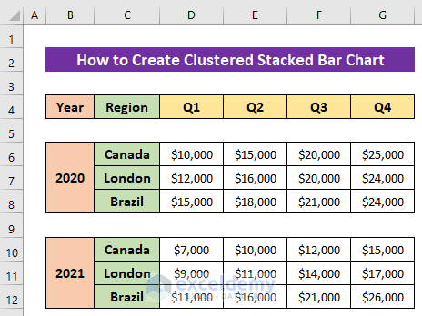
Dataset Overview
Let’s assume we have a dataset representing quarterly sales for a company in three regions over two years.
Steps:
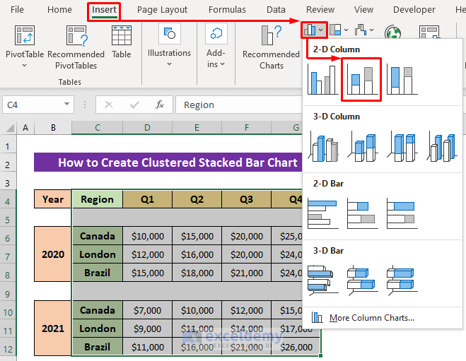
- Select the data range (e.g., C4:G12) that you want to use for your chart.
- Go to the Insert tab.
- Choose Column or Bar Chart and select Stacked Column.
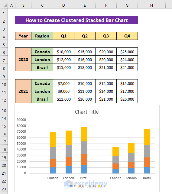
- Once the stacked column chart appears on your sheet, you can further customize it to enhance its appearance and readability.
Customizations for Your Clustered Stacked Bar Chart
Let’s explore some essential customizations:
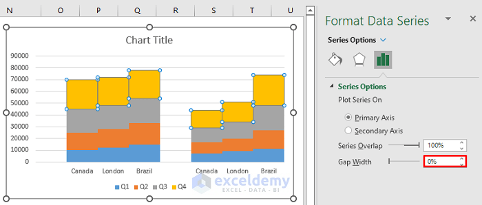
Changing Column Gap Width
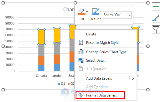
- To adjust the gap between columns within a cluster:
- Right-click on any cluster.
- Select Format Data Series from the context menu.
-
- In the formatting field on the right side of your Excel window, set the gap width to 0%.
-
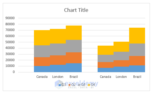
- This eliminates gaps between columns, resulting in continuous clustered columns.
Read More: Excel Chart Bar Width Too Thin
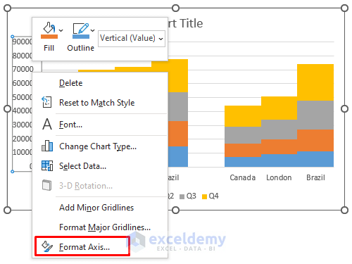
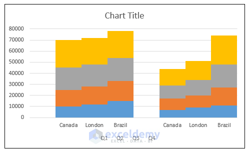
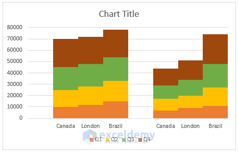
Formatting the Vertical Axis
- Modify the vertical axis to control axis limits, major and minor units, etc.:
- Right-click on the vertical axis.
- Choose Format Axis.
-
- Set the minimum and maximum limits (e.g., maximum limit of 80000).
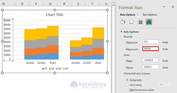
The customized chart will look like the image below:
Read More: How to Make a Simple Bar Graph in Excel
Changing Chart Design
- Excel offers various chart designs:
- Click anywhere on the chart.
- Go to the Chart Design ribbon and select a design from the Chart Styles section.
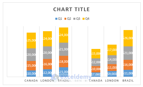
- For example, choose Style 2 to display values within the clusters.
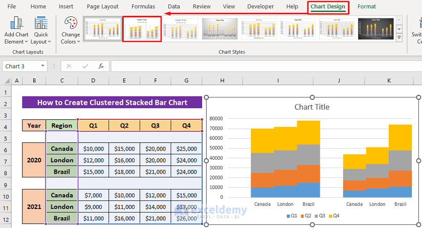
This design shows the values in the cluster.
Read More: How to Make a Diverging Stacked Bar Chart in Excel
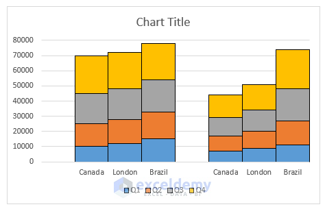
Changing Colors
- Customize column colors to make your chart visually appealing:
- Click anywhere on the chart.
- Navigate to Chart Design > Change Colors.
- Select your desired color scheme (e.g., Colorful Palette 3).
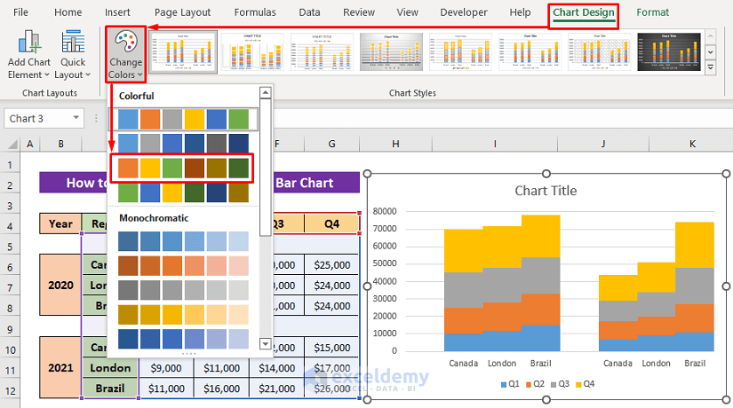
The color of the chart has changed according to our selection.
Read More: How to Change Bar Chart Color Based on Category in Excel
Editing Cluster Borders
- Adding borders to clusters improves clarity:
- Follow the steps from the Changing Column Gap Width section.
- Click on the Fill & Line icon.
- Choose a color for the border (e.g., black).
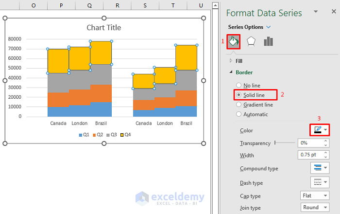
The selected clusters have black borders.
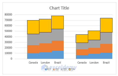
-
- Repeat for other clusters.
Read More: How to Make a 100 Percent Stacked Bar Chart in Excel
You can download the practice workbook from here:
Related Articles
- How to Make a Bar Graph in Excel without Numbers
- How to Create a Bar Chart in Excel with Multiple Bars
- How to Make a Grouped Bar Chart in Excel
- How to Make a Double Bar Graph in Excel
<< Go Back to Stacked Bar Chart in Excel | Excel Bar Chart | Excel Charts | Learn Excel
Get FREE Advanced Excel Exercises with Solutions!
